Download
1 / 52
520 likes | 648 Vues
Modelling Longitudinal Data. General Points Single Event histories (survival analysis) Multiple Event histories. Motivation. Attempt to go beyond more simple material in the first workshop. Begin to develop an appreciation of the notation associated with these techniques.

E N D
Modelling Longitudinal Data • General Points • Single Event histories (survival analysis) • Multiple Event histories
Motivation • Attempt to go beyond more simple material in the first workshop. • Begin to develop an appreciation of the notation associated with these techniques. • Gain a little “hands-on” experience.
Statistical Modelling FrameworkGeneralized Linear Models An interest in generalized linear models is richly rewarded. Not only does it bring together a wealth of interesting theoretical problems but it also encourages an ease of data analysis sadly lacking from traditional statistics….an added bonus of the glm approach is the insight provided by embedding a problem in a wider context. This in itself encourages a more critical approach to data analysis. Gilchrist, R. (1985) ‘Introduction: GLIM and Generalized Linear Models’, Springer Verlag Lecture Notes in Statistics, 32, pp.1-5.
Statistical Modelling • Know your data. • Start and be guided by ‘substantive theory’. • Start with simple techniques (these might suffice). • Remember John Tukey! • Practice.
Willet and Singer (1995) conclude that discrete-time methods are generally considered to be simpler and more comprehensible, however, mastery of discrete-time methods facilitates a transition to continuous-time approaches should that be required.Willet, J. and Singer, J. (1995) Investigating Onset, Cessation, Relapse, and Recovery: Using Discrete-Time Survival Analysis to Examine the Occurrence and Timing of Critical Events. In J. Gottman (ed) The Analysis of Change (Hove: Lawrence Erlbaum Associates).
As social scientists we are often substantively interested in whether a specific event has occurred.
Survival Data – Time to an event In the medical area… • Time from diagnosis to death. • Duration from treatment to full health. • Time to return of pain after taking a pain killer.
Survival Data – Time to an event Social Sciences… • Duration of unemployment. • Duration of housing tenure. • Duration of marriage. • Time to conception. • Time to orgasm.
Consider a binary outcome or two-state event 0 = Event has not occurred 1 = Event has occurred
A 0 1 B 1 0 C 1 0 t1 t2 t3 End of Study Start of Study
These durations are a continuous Y so why can’t we use standard regression techniques?
These durations are a continuous Y so why can’t we use standard regression techniques? We can. It might be better to model the log of Y however. These models are sometimes known as ‘accelerated life models’.
1946 Birth Cohort Study Research Project 2060 (1st August 2032 VG retires!) 1946 A 0 1 B 1 0 C 1 0 t1 t2 t3 t4 Start of Study 1=Death
Breast Feeding Study –Data Collection Strategy1. Retrospective questioning of mothers2. Data collected by Midwives 3. Health Visitor and G.P. Record
Breast Feeding Study – 2001 Age 6 Start of Study Birth 1995
Breast Feeding Study – 2001 0 1 Age 6 1 0 1 0 t1 t2 t3 Start of Study Birth 1995
Accelerated Life Model Loge ti = b0 + b1x1i+ei
Accelerated Life Model error term Beware this is log t explanatory variable Loge ti = b0+ b1x1i+ei constant
At this point something should dawn on you – like fish scales falling from your eyes – like pennies from Heaven.
b0 + b1x1i+ei is the r.h.s. Think about the l.h.s. • Yi - Standard liner model • Loge(odds) Yi - Standard logistic model • Loge ti - Accelerated life model We can think of these as a single ‘class’ of models and (with a little care) can interpret them in a similar fashion (as Ian Diamond of the ESRC would say “this is phenomenally groovy”).
0 1 0 0 1 CENSORED OBSERVATIONS 1 0 1 0 Start of Study End of Study
A 1 B CENSORED OBSERVATIONS Start of Study End of Study
These durations are a continuous Y so why can’t we use standard regression techniques? What should be the value of Y for person A and person B at the end of our study (when we fit the model)?
Cox Regression(proportional hazard model) is a method for modelling time-to-event data in the presence of censored cases. Explanatory variables in your model (continuous and categorical). Estimated coefficients for each of the covariates. Handles the censored cases correctly.
Cox, D.R. (1972) ‘Regression models and life tables’ JRSS,B, 34 pp.187-220.
Childcare Study –Studying a cohort of women who returned to work after having their first child. • 24 month study • The focus of the study was childcare spell #2 • 341 Mothers (and babies)
Variables • ID • Start of childcare spell #2 (month) • End of childcare spell #2 (month) • Gender of baby (male; female) • Type of care spell #2 (a relative; childminder; nursery) • Family income (crude measure)
Describes the decline in the size of the risk set over time. Survival Function (or survival curve)
S(t) = 1 – F(t) = Prob (T>t)alsoS(t1) S(t2) for all t2 > t1 Survival Function
S(t) = 1 – F(t) = Prob (T>t) survival probability Cumulative probability event Survival Function time complement
S(t1) S(t2) for all t2 > t1 All this means is… once you’ve left the risk set you can’t return!!! Survival Function
HAZARD In advanced analyses researchers sometimes examine the shape of something called the hazard. In essence the shape of this is not constrained like the survival function. Therefore it can potentially tell us something about the social process that is taking place.
For the very keen… Hazard – the rate at which events occur Or the risk of an event occurring at a particular time, given that it has not happened before t
For the even more keen… Hazard – The conditional probability of an event occurring at time t given that it has not happened before. If we call the hazard function h(t) and the pdf for the duration f(t) Then, h(t)= f(t)/S(t)
A Statistical Model Y variable = duration with censored observations X1 X2 X3
A Statistical Model Family income Y variable = duration with censored observations Gender of baby Type of childcare Mother’s age A continuous covariate
For the keen..Cox Proportional Hazard Model h(t)=h0(t)exp(bx)
Cox Proportional Hazard Model exponential X var estimate h(t)=h0(t)exp(bx) hazard baseline hazard(unknown)
For the very keen..Cox Proportional Hazard Model can be transformed into an additive model log h(t)=a(t) + bx Therefore…
For the very keen..Cox Proportional Hazard Model log h(t)=b0(t) + b1 x1 This should look distressingly familiar!
Define the code for the event (i.e. 1 if occurred – 0 if censored)
Enter explanatory variables (dummies and continuous)
Chi-square related X var Standard error Estimate Un-logged estimate
What does this mean? Our Y the duration of childcare spell #2. Note we are modelling the hazard!