Download

1 / 35
370 likes | 615 Vues
Ricardian Model. INTERNATIONAL ECONOMICS, ECO 486 JDE notes to supplement the text. David Ricardo April 18, 1772 — September 11, 1823 . Learning Objectives. Understand five more assumptions Determine and understand comparative and absolute advantage Find international trade equilibrium

E N D
Ricardian Model • INTERNATIONAL ECONOMICS,ECO 486 • JDE notes to supplement the text. David Ricardo April 18, 1772 — September 11, 1823
Learning Objectives • Understand five more assumptions • Determine and understand comparative and absolute advantage • Find international trade equilibrium • Explain gains from trade • Derive range of wages that will permit trade
Assumptions • #8 -- Factors of production cannot move between countries • #9 -- There are no barriers to trade in goods.
Assumptions #10 • #10 -- Exports must pay for imports • Assumptions 8-10 apply to both the Classical and HO Models • Assumptions 11 & 12 apply only to Classical Model
Assumptions • #11 -- Labor is the only relevant factor of production in terms of productivity analysis or costs of production. • #12 -- Production exhibits constant returns to scale, CRS,between labor and output. • If both inputs, K & L, are doubled, output doubles • Implies Linear PPF and complete specialization
Ricardian Theorem • A country exports that good which has higher comparative factor productivity and imports the commodity which has lower comparative factor productivity than the other country. • Page 48, Ravendra N. Batra, Studies in the Pure Theory of International Trade
Production possibility frontiers: (a) country A; (b) country B.
Autarky • Given perfect competition, • P = MC • Autarky price of S (on x-axis) equals slope of PPF • Resource payments correspond to their productivity
Absolute Advantage • Compare one good across countries. • Country with greater output per labor hour has an absolute advantage in that good.
Comparative Advantage • Calculate opportunity costs. • Compare one good across countries. • Country with lower opportunity cost has a comparative advantage in that good.
Which Advantage? • Absolute advantage is a special case. • Comparative advantage is the general case.
Terms of Trade • Once trade begins, an international equilibrium results • Results in one world price for a good
International Trade Equilibrium • Complete specialization in Comparative Advantage good • CIC & ToT tangent at consumption point • Congruent trade triangles imply balanced trade
Gains From Trade • More of both goods attainable • GDP increases at pre-trade prices • Higher CIC is attainable
Exchange Rates • State exchange rate, E, in US dollars per UK pound • say $2/£ • A good will be imported if its foreign pre-trade price (x E) is less than the domestic price • PS < E x PS*
Buy Low . . . • Trade requires • PS < E x PS* • PT > E x PT* • autarky prices • Home (A) has comparative advantage in S • Foreign (B) has comparative advantage in T
Perfect Competition Review(Product & Resource Markets) • PX = MC for a good, X • MC = w/MPPL (Labor, L, is only var. input) • w=MRPL =(MR) MPPL=(P) MPPL=VMPL
Prices & Wages • PX = MC = w/MPPL • MPPL is measured as units of X per hour, OLX • Productivity may be stated as hours per unit of X, aLX, or units of X per hour worked, OLX. aLX = 1/OLX • PX = w /OLX
Competitive Advantage • The ability to sell a good at the lowest price. • Usually results from comparative advantage • Alternatively, it may be the result of . . . • Government subsidies for inefficient industries • An undervalued exchange rate
Losing Competitive Advantage • If Home’s relative wage ratio (W/W*) exceeds its relative productivity (OLS/OLS*), its S will cost _______ than Foreign’s. • If a country’s currency is overvalued (say $1/£ instead of $2/£), comparative advantage may be lost -- both goods may be cheaper in ___________.
Cambodian Textiles Update • US offered to expand Cambodia’s export quota by 14% if “working conditions is the Cambodia textile and apparel sector substantially comply with” local and internationally recognized core standards. • Dec ’99 – US officials decide that Cambodia has fallen short, but offered 5% • Cambodia to establish independent monitoring with the International Labor Organization, ILO
Cambodian Textiles Update • ILO leery, fearing weakening of local monitoring capability • ILO agrees after US pledges $500,000 in technical assistance to Cambodian labor ministry • US also paying $1 million (of $1.4 mil.) for a 3-year monitoring effort • USTR press release 18 May 2000
Cambodian Textiles Update • Sep ’00 – US officials grant Cambodia another 4% increase • 9% increase continued for ’01 • Other news: • Nov ’00 -- ILO rules Burma’s progress on forced labor inadequate. Section 33 action authorized. As of March ’01, no member country has taken action. US & EU considering sanctions • Bush proposed reducing US contributions to the ILO budget.
Quantity of Soybeans Demanded PS/PT = 2.5 yd.T/bu.S 10 H Autarky General Equilibrium|slope PPF| = PS/PT =2 yd.T/bu.S 8 G TEXTILES, T (millions of yards per year) 6 L PS/PT = 1 yd.T/bu.S 4 CIC2 2 CIC1 CIC0 PPF 1.8 0 2 4 6 8 10 4.7 SOYBEANS, S (millions of bushels per year)