Download
1 / 15
180 likes | 396 Vues
Chapter 3- Matrices LECTURE 5. Prof. Dr. Zafer ASLAN. MATRICES. Introduction

E N D
Chapter 3- Matrices LECTURE5 Prof. Dr. Zafer ASLAN
MATRICES Introduction In working with a system of linear equations, only the coefficients and their respective positions are important. Also, in reducing the system to echelon form, it is essential to keep the equations carefully aligned. Thus these coefficients can be efficiently arranged in rectangular array called a “matrix”. Matrices: Let K be an arbitrary field. A rectangular array of the form: Where the aij are scalars in K, is called a matrix over K, or simply a matrix if K is implicit.
MATRICES Matrices Let K be an arbitrary field. A rectangular array of the form: Where the aij are scalars in K, is called a matrix over K, or simply a matrix if K is implicit. is the row of the matrix, and; is its column. Note that the element aij, called ij-entry or ij – component, appears in the ith row and the jth column. A matrix with m rows and n columns is called an m by n (or mxn) matrix. The pair of numbers (m,n) is called its size or shape.
MATRICES Matrix Addition and Scalar Multiplication Let A and B be two matrices with the same size, i.e. The same number of rows and of columns, say mxn matrices:
MATRICES THEOREM 3.1. Let V be the set of all mxn matrices over a field K. Then for any matrices A,B,C V and any scalars k1, k2 K, i) (A+B)+C = A+(B+C) ii) A+0=A iii) A+(-A)=0 iv) A+B=B+A v) k1(A+B) = k1A +k1B vi) (k1+k2)A=k1A+k2A vii) (k1k2)A=k1(k2A) viii) 1.A=A and 0A=0 Observe that A+B and kA are also mxn matrices. We also define; -A = -1.A and A – B = A+ (-B) The sum of matrices with different sizes is not defined.
MATRICES Matrix Addition and Scalar Multiplication The sum of A and B, written A+B, is the matrix obtained by adding corresponding entries:
MATRICES Matrix Addition and Scalar Multiplication The product of a scalar k by the matrix A, written k.A or simply kA, is the matrix obtained by multiplying each entry of A by k: Observe that A+B and kA are also mxn matrices. We also define; -A = -1.A and A – B = A+ (-B) The sum of matrices with different sizes is not defined.
MATRICES THEOREM 3.1. Let V be the set of all mxn matrices over a field K. Then for any matrices A,B,C V and any scalars k1, k2 K, i) (A+B)+C = A+(B+C) ii) A+0=A iii) A+(-A)=0 iv) A+B=B+A v) k1(A+B) = k1A +k1B vi) (k1+k2)A=k1A+k2A vii) (k1k2)A=k1(k2A) viii) 1.A=A and 0A=0
MATRICES MATRIX MULTIPLICATION Consider the equations: a11y1 + a12 y2 = z1 a21y1 + a22 y2 = z2 We can present the matrix equation: AY = Z
MATRICES THEOREM 3.2. i) (AB)C=A(BC) (associative law) ii) A(B+C)=AB+AC (left distributive law) iii) (B+C)A=BA+CA (right distributive law) iv) k(AB)=(kA)B=A(kB) (where k is a scalar. Observe that A+B and kA are also mxn matrices. We also define; -A = -1.A and A – B = A+ (-B) The sum of matrices with different sizes is not defined.
MATRICES TRANSPOSE The transpose of a matrix A, written At, is the matrix obtained by writing the rows of A, in order, as columns:
MATRICES ECHELON MATRICES A matrix A=(aij) is an echelon matrix, or is said to be in echelon form, if the number of zeros preceding the first nonzero entry of a row, increases row by row until only zero rows remain, that is if there exists nonzero entries. Algorithm which row reduces a matrix to echelon form: Step 1. Suppose the j1 column is the first column with a nonzero entry. Interchange the rows to that this nonzero entry appears in the first row, that is so that a1j10 Step 2. For each i>1, apply the operation. Rithen –aij1R1 + a1j1R1
MATRICES SQUARE MATRICES A matrix with the same number of rows as columns is called a square matrix. A square matrix with n rows and n columns is said to be order n, and is called an n-square matrix. The diagonal (or main diagonal) of the n-square matrix A = (aij) consists of the elements a11, a22, ... ,ann.
MATRICES INVERTIBLE MATRICES A square matrix A is said to be invertible if there exists a matrix B with the property that; AB = BA = I Where I is the identity matrix. Such a matrix B is unique. We call such a matrix B the inverse of A and denote it by A-1. BLOCK MATRICES Using a system of horizontal and vertical lines, we can partition a matrix A into smaller matrices called blocks(or cells) of A. The matrix A is called a block matrix. A given matrix may be divided into blocks in different ways.
Next Lecture (Week 6) Chapter 4:Vector Spaces and Subspaces Reference Seymour LIPSCHUTZ, (1987): Schaum’s Outline of Theory and Problems of LINEAR ALGEBRA, SI (Metric) Edition, ISBN: 0-07-099012-3, pp. 334, McGraw – Hill Book Co., Singapore.