Download
1 / 37
370 likes | 427 Vues
s c r e e n. s c r e e n. Lecturer’s desk. Row A. Row A. 13. 12. 11. 10. 9. 8. 7. 17. 16. 15. 14. Row A. 19. 18. 4. 3. 2. 1. 6. 5. Row B. 14. 13. 12. 11. 10. 9. 15. Row B. 8. 7. 20. 4. 3. 2. 1. 19. 18. 17. 16. 6. 5. Row B. Row C. 4. 3. 2. 1.

E N D
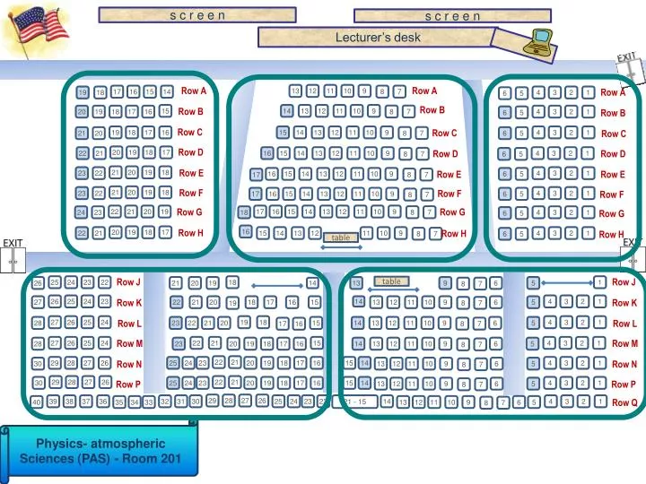
s c r e e n s c r e e n Lecturer’s desk Row A Row A 13 12 11 10 9 8 7 17 16 15 14 Row A 19 18 4 3 2 1 6 5 Row B 14 13 12 11 10 9 15 Row B 8 7 20 4 3 2 1 19 18 17 16 6 5 Row B Row C 4 3 2 1 15 14 13 12 11 10 9 19 18 17 16 Row C 8 7 6 5 21 20 Row C Row D 20 19 18 17 22 21 4 3 2 1 16 15 14 13 12 11 10 9 Row D Row D 8 7 6 5 21 20 19 18 Row E 23 22 4 3 2 1 6 5 16 15 14 13 12 11 10 9 Row E Row E 8 7 17 21 20 19 18 Row F 23 22 4 3 2 1 Row F 6 5 17 16 15 14 13 12 11 10 9 Row F 8 7 22 21 20 19 17 16 15 14 13 12 11 10 9 Row G Row G 8 7 24 23 18 4 3 2 1 6 5 Row G 16 20 19 18 17 Row H 22 21 4 3 2 1 15 14 13 12 11 10 9 Row H 8 7 6 5 Row H table Row J Row J 25 24 23 22 1 18 table 9 6 26 5 20 19 21 13 8 7 14 26 25 24 23 4 3 2 1 27 5 20 22 21 14 13 12 11 10 9 6 18 17 16 15 Row K Row K 8 7 19 27 26 25 24 4 3 2 1 19 18 28 5 20 23 22 21 14 13 12 11 10 9 6 15 Row L Row L 8 7 17 16 4 3 2 1 27 26 25 24 22 21 15 Row M Row M 5 28 23 20 19 14 13 12 11 10 9 6 18 17 16 8 7 22 21 29 28 27 26 4 3 2 1 20 23 19 15 14 18 17 16 25 24 30 5 13 12 11 10 9 6 Row N Row N 8 7 29 28 27 26 22 21 30 4 3 2 1 20 23 19 15 14 18 17 16 25 24 5 13 12 11 10 9 6 Row P Row P 8 7 29 28 27 26 39 38 37 36 30 4 3 2 1 32 31 23 22 21 - 15 14 25 24 40 5 33 35 34 13 12 11 10 9 6 Row Q 8 7 Physics- atmospheric Sciences (PAS) - Room 201
Introduction to Statistics for the Social SciencesSBS200, COMM200, GEOG200, PA200, POL200, or SOC200Lecture Section 001, Fall, 2012Room 201 Physics and Atmospheric Sciences (PAS)10:00 - 10:50 Mondays, Wednesdays & Fridays. Welcome Please double check – Allcell phones other electronic devices are turned off and stowed away http://www.youtube.com/watch?v=oSQJP40PcGI
Schedule of readings Before next exam – This Friday (November 9th) Please read chapters 7 - 14 Please read Chapters 2, 3, and 4 in Plous Chapter 2: Cognitive Dissonance Chapter 3: Memory and Hindsight Bias Chapter 4: Context Dependence Study Guide is on class website
Lab sessions Labs continuethis week with Exam Reviews
Please click in My last name starts with a letter somewhere between A. A – D B. E – L C. M – R D. S – Z
Use this as your study guide By the end of lecture today11/5/12 Analysis of Variance Logic of hypothesis testing Steps for hypothesis testing Hypothesis testing with ANOVAs Constructing brief, complete summary statements Preparing for Exam 3
Homework due – Wednesday (November 7th) • Assignment 20 - Construct Quiz Items: • Please write 3 multiple choice questions based on any lecture since last exam (October 12). • Bring two copies to class. • Each multiple choice question must contain: • a person’s name, • only one correct answer, • and 3 incorrect options for a total of 4 options for each question
Type of major in school 4 (accounting, finance, hr, marketing) Grade Point Average Homework 0.05 2.83 3.02 3.24 3.37
0.3937 0.1119 If observed F is bigger than critical F:Reject null & Significant! If observed F is bigger than critical F:Reject null & Significant! 0.3937 / 0.1119 = 3.517 Homework 3.517 3.009 If p value is less than 0.05:Reject null & Significant! 3 24 0.03 4-1=3 # groups - 1 # scores - number of groups 28 - 4=24 # scores - 1 28 - 1=27
Yes Homework = 3.517; p < 0.05 F (3, 24) The GPA for four majors was compared. The average GPA was 2.83 for accounting, 3.02 for finance, 3.24 for HR, and 3.37 for marketing. An ANOVA was conducted and there is a significant difference in GPA for these four groups (F(3,24) = 3.52; p < 0.05).
Average for each group(We REALLY care about this one) Number of observations in each group Just add up all scores (we don’t really care about this one)
Number of groups minus one(k – 1) 4-1=3 “SS” = “Sum of Squares”- will be given for exams Number of people minus number of groups (n – k) 28-4=24
SS between df between SS within df within MS between MS within
Type of executive 3 (banking, retail, insurance) Hours spent at computer 0.05 10.8 8 8.4
11.46 2 If observed F is bigger than critical F:Reject null & Significant! If observed F is bigger than critical F:Reject null & Significant! 11.46 / 2 = 5.733 5.733 3.88 If p value is less than 0.05:Reject null & Significant! 2 12 0.0179
Yes p < 0.05 F (2, 12) = 5.73; The number of hours spent at the computer was compared for three types of executives. The average hours spent was 10.8 for banking executives, 8 for retail executives, and 8.4 for insurance executives. An ANOVA was conducted and we found a significant difference in the average number of hours spent at the computer for these three groups , (F(2,12) = 5.73; p < 0.05).
Average for each group(We REALLY care about this one) Number of observations in each group Just add up all scores (we don’t really care about this one)
Number of groups minus one(k – 1) 3-1=2 “SS” = “Sum of Squares”- will be given for exams Number of people minus number of groups (n – k) 15-3=12
SS between df between SS within df within MS between MS within
Five steps to hypothesis testing Step 1: Identify the research problem (hypothesis) Describe the null and alternative hypotheses Step 2: Decision rule • Alpha level? (α= .05 or .01)? Still, difference between means • Critical statistic (e.g. z or t or F or r) value? Step 3: Calculations MSBetween F = MSWithin Still, variabilityof curve(s) Step 4: Make decision whether or not to reject null hypothesis If observed t (or F) is bigger then critical t (or F) then reject null Step 5: Conclusion - tie findings back in to research problem
Comparing ANOVAs with t-tests Similarities still include: Using distributions to make decisions about common and rare events Using distributions to make inferences about whether to reject the null hypothesis or not The same 5 steps for testing an hypothesis Tells us generally about number of participants / observations Tells us generally about number of groups / levels of IV • The three primary differences between t-tests and ANOVAS are: • 1. ANOVAs can test more than two means • 2. We are comparing sample means indirectly by • comparing sample variances • 3. We now will have two types of degrees of freedom • t(16) = 3.0; p < 0.05 F(2, 15) = 3.0; p < 0.05 Tells us generally about number of participants / observations
One way analysis of varianceVariability is divided Remember, one-way = one IV Number of cookies sold None Bike Hawaii trip Incentives Total variability Between group variability (only one factor) Within group variability (error variance) This will be our numerator – like difference between means This will be our denominator – like within group variabilityRemember, error variance = random error
Sum of squares (SS): The sum of squared deviations of some set of scores about their mean Mean squares (MS): The sum of squares divided by its degrees of freedom Mean square between groups: sum of squares between groups divided by its degrees of freedom Mean square total: sum of squares total divided by its degrees of freedom MSBetween F = Mean square within groups: sum of squares within groups divided by its degrees of freedom MSWithin Note: MStotal= MSwithin+ MSbetween
. Effect size is considered relativeto variability of distributions Treatment Effect x Variability between groups Treatment Effect x Variabilitywithin groups
ANOVA Variability between groups F = Variability within groups Variability Between Groups “Between” variability bigger than “within” variability so should get a big (significant) F Variability Within Groups Variability Within Groups Variability Between Groups “Between” variability getting smaller “within” variability staying same so, should get a smaller F Variability Within Groups Variability Within Groups Variability Between Groups “Between” variability getting very small “within” variability staying same so, should get a very small F Variability Within Groups Variability Within Groups
ANOVA Variability between groups F = Variability within groups Variability Between Groups “Between” variability bigger than “within” variability so should get a big (significant) F Variability Within Groups Variability Within Groups Variability Between Groups “Between” variability getting smaller “within” variability staying same so, should get a smaller F Variability Within Groups “Between” variability getting very small “within” variability staying same so, should get a very small F (equal to 1)
MSbetween MSwithin 40 88 SSbetween 12 2 dfbetween 3-1=2 # groups - 1 SSwithin dfwithin # scores - number of groups 15-3=12 88 20 =2.73 =7.33 40 # scores - 1 7.33 12 =20 2 15- 1=14
No, so it is not significant Do not reject null No, so it is not significant Do not reject null F critical(is observed F greater than critical F?) P-value(is it less than .05?)
How to report the findings for an ANOVA One paragraph summary of this study. Describe the IV & DV, and present the means, which type of test was conducted, and the statistical results. Start summary with two means (based on DV) for two levels of the IV The average number of cookies sold for three different incentives were compared. The mean number of cookie boxes sold for the “Hawaii” incentive was 14 , the mean number of cookies boxes sold for the “Bicycle” incentive was 12, and the mean number of cookies sold for the “No” incentive was 10. An ANOVA was conducted and there appears to be no significant difference in the number of cookies sold as a result of the different levels of incentive F(2, 12) = 2.73; n.s. Type of test with degrees of freedom Describe type of test (t-test versus anova) with brief overview of results Value of observed statistic p<0.05 = “significant”
Review for Exam 3
Thank you! See you next time!!