Download
1 / 48
490 likes | 634 Vues
ENA measurements of the ring current. Robert DeMajistre. Overview. Motivation for ENA imaging Measurement mechanism The HENA instrument HENA measurements/retrievals Validation Results The next steps. In situ measurements Cluster observation of the ring current Precise measurements

E N D
ENA measurements of the ring current Robert DeMajistre
Overview • Motivation for ENA imaging • Measurement mechanism • The HENA instrument • HENA measurements/retrievals • Validation • Results • The next steps
In situ measurements • Cluster observation of the ring current • Precise measurements • Lack of global context – single trace through a 4 dimensional structure (3 space, time)
Global context • In situ measurements often alias space and time • Overall morphology is difficult to deduce • Multiple spacecraft help • Statistical models are difficult to assemble • Combination of precise in situ measurements and qualitative morphology very attractive • ENA imaging to the rescue
IMAGE geometry (geographic)
+ - - + + - - + + - - + + - - + + - - High Energy Neutral Atom Imager
Example HENA Image Earth disk Clock Angle Magnetic field lines Particle brightness is represented in false color Direction to Sun
Retrieval Method • Transform spatial integral into dipole coordinates (L, f, m), expand pitch angle dependence in Legendre polynomials • Use 2-D linear quadrature to convert to linear equations • Use 2-D constrained least squares to solve
Tuning inputs Simulated image from October 4, 2000
TuningResults • Second difference (H2) provides better quantitative agreement at the peak • Markov provides better overall morphology • In practice, we combine the two
Selected Results • Ring current peak is often observed at midnight (or later) rather than at the ‘classical’ position at dusk • Dipolarizations and depletions (observed) in time series – clues to how substorms develop
~100-150 keV Oxygen | 40-50 keV Hydrogen March 31, 2001
Next steps • TWINS • Dual vantage point • Earth looking • Launches in 06 and 07 • Casini/INCA • Currently orbiting Saturn • Good data on both Saturn and Titan
Conclusion • ENA imaging is giving us a new view into ring current morphology • We’ve improved our insight into the storm time behavior of the magnetosphere • In coordination with the in situ instruments we can make important quantitative statements about how the magnetosphere behaves.
Overview • Remote sensing – what and why • Mathematical framework for inverse problems • Case studies: • Nighttime electron density inferred from ultraviolet emission measurements (TIMED/GUVI) • Atmospheric composition inferred from Stellar Occultation Measurements (MSX/UVISI) • Ion intensities inferred from Energetic Neutral Atom (ENA) imaging (IMAGE/HENA) • System engineering implications
What? Making measurements where the instrument does not have direct physical access to the object of measurement Why? Many problems in space science require measurement of multiple locations nearly simultaneously – costs of sufficient in situ measurements are prohibitive
Remote sensing is indirect y=F[X;P] Forwardmodel Inversemodel X=F-1[y;P]
Problems with using exact inverse y=F[X;P] X=F-1[y;P] • Solution may not exist • Only for an EOM in specific forms • It may not be unique – many x may produce a single y • It may be poorly conditioned – slightly different x may yield different y • Measurement noise is always present • Pose a similar problem that can be solved more easily
Example of direct retrieval I=Kh • Simplified example – similar to recombination problem • Linear problem • Noise added to measurement • Noise amplification very noticeable (poorly conditioned) • Only marginally acceptable results
The least squares alternative • Instead of exact solution, search for the values of x that are most consistent with the measurement • Minimize the square (epTSy-1ep) of the prediction error ep=y-F(x;p)weighted bythe inverse ofSy(the measurement covariance) • There are standard solutions for linear problems (e.g., Bevington) • Even moderately nonlinear problems can be solved iteratively
Adding information • The least squares solution is likely to be just as ill conditioned as is the direct solution • Adding measurements is not very effective (~N-1/2) • Additional physical information must be introduced to stabilize the inversion
Constrained inversions • MinimizeepTSy-1ep+gxTHxwhere the matrix H is chosen with the expectation that xTHx should be small. The tuning parameter gmodulates the influence of the constraint • Example – if we expect x to be smooth, we could put H=D1TD1,where D1is the first derivative operator
Constraints in perspective • Constraints add information to the problem • Can be formally equivalent to additional measurements • H and g quantify the character of these constraints (y-Kx)Ts-2(y-Kx)+gxDTDx
Constraints • Constraints can dramatically reduce error amplification • They can also introduce significant systematic errors • Prediction error ALWAYS increases • Relying on information in addition to the actual measurements
Metrics for tuning constraints • Tune through simulation • cr2=(1/Ny) epTSy-1ep– does the data fit the model • g =(1/Nx)(xm-xs)T Sx-1(xm-xs)– does the retrieval match the input to the simulation • q=(cr2 -1)2+(g-1)2 • Minimize q
EOM for space based measurements • Many measurement systems can be represented by a common physical model • Though mechanisms vary, the formal similarity is striking • Two essential parts • Instrument equation • Equation of transfer
Equation of transfer • Applicable to a wide variety of information carries: • Photons • Massive particles in tenuous media Transmission from 0 to s Transmission from s’ to s s ò ¢ ¢ ¢ = + I ( s ; E ) I ( 0 ; E ) T ( s , 0 ; E ) J ( s ; E ) T ( s , s ; E ) d s 0 Intensity at s Intensity at 0 Source at s’
Instrument equation • Covers most instrument effects • Non-linearity neglected for now • Assumes instrument measures local intensity of information carriers Smearing function Background counts in channel i Counts in channel i
Approach to Solution • Cast problem in general form • Replace integrals with discrete quadratures • Linearize the problem (if necessary) • Formulate constraints • Tune the constraints • Validate with independent measurements
Case studies • TIMED/GUVI electron density retrievals – one dimensional, single color, single constituent retrieval (limited by SNR) • MSX/UVISI Stellar occultation – one dimensional, multi-spectral, multi constituent retrieval (limited by SNR and size of data set) • IMAGE/HENA ENA imaging – two dimensional retrieval (limited by SNR and viewing geometry)
Constraint Matrices • Boundary constraint – force solution to be small at boundaries of L • Cylindrical boundary inf • Smoothness constraint with asymmetry parameter • First difference (force solution to be small) • Second difference (force Laplacian to be small) • Markov constraint – force changes to be small over a correlation length • Optimize smoothness strength,g, boundary strength,l, and either asymmetry or correlation length, a – need a method
Impact of ENA measurements • ENA imaging on the IMAGE spacecraft provides the first global view of the inner magnetosphere • The retrievals described here have been used to study global behaviors for the first time • Skewed peak of the ring current density towards midnight • “Dipolarizations” of the ring current during substorms • Growth phase dropouts – “choking off” of the ring current during the growth phase
Common Elements of Case Studies • Similar inversion procedures have been successfully applied to disparate data sets • Problems and solutions are formally similar • Common tuning process for constraints are used • Suggests common solutions in measurement system design • Replace integrals with discrete quadratures • Linearize the problem (if necessary) • Formulate constraints • Tune the constraints • Cast problem in general form • Validate with independent measurements In all cases, retrievals were designed after instrument flight
System Engineering • The tools used for developing retrievals and tuning constraints can also be used as part of instrument design • Forward modeling of the Equation of Measurement • Retrieval sensitivity to instrument parameters • System focus on retrieval accuracy rather than radiometric accuracy • Optimize (quantitatively) instrument tradeoffs based on final retrieval accuracy(e.g., should I sacrifice some SNR for better spectral resolution?)
Measurement System Design • Develop coupled simulation of radiation mechanism and instrument early • Use it to help with instrument and spacecraft tradeoffs • Keep it current as project develops • Alternate lower fidelity models can be developed and compared • Add data system and inversion modules to be used with optimization of instrument • Use these modules to identify and exploit opportunities for in-flight calibration refinement
Calibration and data products • Currently, calibration emphasizes the production of radiances from instrument data (required by NASA) • Shift focus to characterizing full instrument function for use in retrievals. • Shift priority to lower level data products for retrieval team and higher level products for the users (calibrated radiances are almost always of marginal utility)
Science Impacts • Night-side ionosphere • New quiet time maps of the low/midlatitude ionosphere • Basis for studying the quiet time interaction of the thermosphere/ionosphere • Stellar Occultation • Study of ozone behavior during polar night • Study of molecular oxygen and ozone in the mesosphere/thermosphere • ENA • First global quantitative view of the inner magnetosphere • Several storm time phenomena have been observed and studied from a global perspective • Comparisons with models of the inner magnetosphere
Next steps • Night-side ionosphere • SSUSI an instrument similar to (but more sensitive than) GUVI is now in orbit, more are planned • Additional instruments are being proposed focusing on nighttime limb observations • Stellar occultation • Instruments to be proposed include extensions to IR for use at Mars • ENA • Doublestar (now flying )TWINS (near launch) to provide multi-position ENA measurements • Cassini/INCA now at Saturn, IBEX now phase B
Conclusions • We’ve described a general framework for space based remote sensing • Techniques developed here have been used successfully across a broad range of applications • The products resulting from these techniques are being applied to significant and interesting problems • The techniques also allow for more effective system design of remote sensing systems