Download
1 / 24
240 likes | 246 Vues
Introduction to Algorithms Red-Black Trees. CSE 680 Prof. Roger Crawfis. Red-black trees: Overview. Red-black trees are a variation of binary search trees to ensure that the tree is balanced . Height is O (lg n ), where n is the number of nodes.

E N D
Introduction to AlgorithmsRed-Black Trees CSE 680 Prof. Roger Crawfis
Red-black trees: Overview • Red-black trees are a variation of binary search trees to ensure that the tree is balanced. • Height is O(lg n), where n is the number of nodes. • Operations take O(lg n) time in the worst case.
Red-black trees: Overview • Red-black trees are a variation of binary search trees to ensure that the tree is somewhat balanced. • Height is O(lgn), where n is the number of nodes. • Operations take O(lgn) time in the worst case. • Easiest of the balanced search trees, so they are used in STL map operations…
Red-black Tree • Binary search tree + 1 bit per node: the attribute color, which is either red or black. • All other attributes of BSTs are inherited: • key, left, right, and p. • All empty trees (leaves) are colored black. • We use a single sentinel, nil, for all the leaves of red-black tree T, with color[nil] = black. • The root’s parent is also nil[T ].
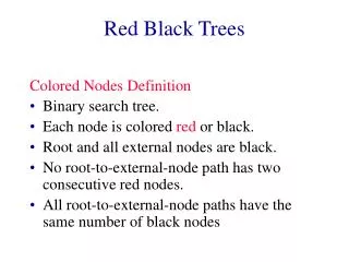
Red-black Properties • Every node is either red or black. • The root is black. • Every leaf (nil) is black. • If a node is red, then both its children are black. • For each node, all paths from the node to descendant leaves contain the same number of black nodes.
nil[T] Red-black Tree – Example 26 Remember: every internal node has two children, even though nil leaves are not usually shown. 17 41 30 47 38 50
Height of a Red-black Tree • Height of a node: • h(x) = number of edges in a longest path to a leaf. • Black-height of a node x, bh(x): • bh(x)= number of black nodes (including nil[T ]) on the path from x to leaf, not counting x. • Black-height of a red-black tree is the black-height of its root. • By Property 5, black height is well defined.
Example: Height of a node: h(x) = # of edges in a longest path to a leaf. Black-height of a node bh(x)= # of black nodes on path from x to leaf, not counting x. How are they related? bh(x) ≤h(x) ≤ 2 bh(x) Height of a Red-black Tree h=4 bh=2 26 h=3 bh=2 h=1 bh=1 17 41 h=2 bh=1 h=2 bh=1 30 47 h=1 bh=1 38 h=1 bh=1 50 nil[T]
Lemma “RB Height” Consider a node x in an RB tree: The longest descending path from x to a leaf has length h(x), which is at most twice the length of the shortest descending path from x to a leaf. Proof: # black nodes on any path from x = bh(x) (prop 5) • # nodes on shortest path from x, s(x). (prop 1) But, there are no consecutive red (prop 4), and we end with black (prop 3), so h(x) ≤ 2 bh(x). Thus, h(x) ≤ 2 s(x).QED
Bound on RB Tree Height • Lemma 13.1: A red-black tree with n internal nodes has height at most 2 lg(n+1).
Left-Rotate(T, x) y x x Right-Rotate(T, y) y Rotations
Left-Rotate(T, x) y x x Right-Rotate(T, y) y Rotations • Rotations are the basic tree-restructuring operation for almost all balanced search trees. • Rotation takes a red-black-tree and a node, • Changes pointers to change the local structure, and • Won’t violate the binary-search-tree property. • Left rotation and right rotation are inverses.
Left-Rotate(T, x) y x Right-Rotate(T, y) x y Left Rotation – Pseudo-code Left-Rotate (T, x) • y right[x] // Set y. • right[x] left[y] //Turn y’s left subtree into x’s right subtree. • if left[y] nil[T ] • then p[left[y]] x • p[y] p[x] // Link x’s parent to y. • if p[x] = nil[T ] • then root[T ] y • else if x = left[p[x]] • then left[p[x]] y • else right[p[x]] y • left[y] x // Put x on y’s left. • p[x] y
Rotation • The pseudo-code for Left-Rotate assumes that • right[x] nil[T ], and • root’s parent is nil[T ]. • Left Rotation on x, makes x the left child of y, and the left subtree of y into the right subtree of x. • Pseudocode for Right-Rotate is symmetric: exchange left and right everywhere. • Time:O(1)for both Left-Rotate and Right-Rotate, since a constant number of pointers are modified.
Reminder: Red-black Properties • Every node is either red or black. • The root is black. • Every leaf (nil) is black. • If a node is red, then both its children are black. • For each node, all paths from the node to descendant leaves contain the same number of black nodes.
Insertion in RB Trees • Insertion must preserve all red-black properties. • Should an inserted node be coloredRed? Black? • Basic steps: • Use Tree-Insert from BST (slightly modified) to insert a node x into T. • Procedure RB-Insert(x). • Color the node x red. • Fix the modified tree by re-coloring nodes and performing rotation to preserve RB tree property. • Procedure RB-Insert-Fixup.
Insertion – Fixup • Problem: we may have one pair of consecutive reds where we did the insertion. • Solution: rotate it up the tree and away… • Three cases have to be handled…
Insertion – Fixup RB-Insert-Fixup(T, z) • while color[p[z]] = RED • do if p[z] = left[p[p[z]]] • then y right[p[p[z]]] • if color[y] = RED • then color[p[z]] BLACK // Case 1 • color[y] BLACK // Case 1 • color[p[p[z]]] RED // Case 1 • z p[p[z]] // Case 1
Insertion – Fixup RB-Insert-Fixup(T, z)(Contd.) else if z = right[p[z]] // color[y] RED then z p[z] // Case 2 LEFT-ROTATE(T, z)// Case 2 color[p[z]] BLACK // Case 3 color[p[p[z]]] RED // Case 3 RIGHT-ROTATE(T, p[p[z]])// Case 3 else (if p[z] = right[p[p[z]]])(same as 10-14 with “right” and “left” exchanged) color[root[T ]] BLACK
p[p[z]] (z’s grandparent) must be black, since z and p[z] are both red and there are no other violations of property 4. Make p[z] and y black now z and p[z] are not both red. But property 5 might now be violated. Make p[p[z]] red restores property 5. The next iteration has p[p[z]] as the new z (i.e., z moves up 2 levels). Case 1 – uncle y is red p[p[z]] new z C C p[z] y A D A D z B B z is a right child here. Similar steps if z is a left child.
Left rotate around p[z], p[z] and z switch roles now z is a left child, and both z and p[z] are red. Takes us immediately to case 3. Case 2 – y is black, z is a right child C C p[z] p[z] A y B y z z A B
Make p[z] black and p[p[z]] red. Then right rotate on p[p[z]]. Ensures property 4 is maintained. No longer have 2 reds in a row. p[z] is now black no more iterations. Case 3 – y is black, z is a left child B C p[z] A C B y z A
Algorithm Analysis • O(lgn)time to get through RB-Insert up to the call of RB-Insert-Fixup. • Within RB-Insert-Fixup: • Each iteration takes O(1)time. • Each iteration butthe last moves z up 2 levels. • O(lgn)levels O(lgn)time. • Thus, insertion in a red-black tree takes O(lgn)time. • Note: there are at most 2 rotations overall.
Deletion • Deletion, like insertion, should preserve all the RB properties. • The properties that may be violated depends on the color of the deleted node. • Red – OK. • Black? • Steps: • Do regular BST deletion. • Fix any violations of RB properties that may result.