Download
1 / 54
540 likes | 666 Vues
Bond, Boyle, Kofman, Prokushkin, Vaudrevange. Zero Point Gravity Wave Fluctuations from Inflation. Cosmic Probes CMB, CMBpol (E,B modes of polarization) B from tensor: Bicep, Planck, Spider, Spud, Ebex, Quiet, Pappa, Clover, …, Bpol CFHTLS SN(192) , WL(Apr07) , JDEM/DUNE BAO, LSS,Ly a.

E N D
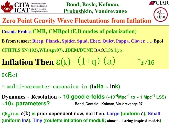
Bond, Boyle, Kofman, Prokushkin, Vaudrevange Zero Point Gravity Wave Fluctuations from Inflation Cosmic Probes CMB, CMBpol (E,B modes of polarization) B from tensor: Bicep, Planck, Spider, Spud, Ebex, Quiet, Pappa, Clover, …, Bpol CFHTLS SN(192),WL(Apr07), JDEM/DUNE BAO,LSS,Lya Inflation Thenk=(1+q)(a) ~r/160< = multi-parameter expansion in (lnHa ~ lnk) Dynamics ~ Resolution~ 10 good e-folds (~10-4Mpc-1 to ~ 1 Mpc-1 LSS) ~10+ parameters? Bond, Contaldi, Kofman, Vaudrevange 07 r(kp) i.e. k is prior dependent now, not then. Large (uniform ), Small (uniform ln). Tiny (roulette inflation of moduli; almost all string-inspired models) KKLMMT etc, Quevedo etal, Bond, Kofman, Prokushkin, Vaudrevange 07, Kallosh and Linde 07 General argument: if the inflaton < the Planck mass, then r < .01 (Lyth96 bound)
CBI pol to Apr’05 Quiet2 Bicep CBI2 to Dec’07 (1000 HEMTs) Chile QUaD Quiet1 Acbar to Jan’06 SCUBA2 APEX Spider (12000 bolometers) (~400 bolometers) Chile SZA JCMT, Hawaii (2312 bolometer LDB) (Interferometer) California ACT Clover (3000 bolometers) Chile Boom03 2017 CMBpol 2003 2005 2007 2004 2006 2008 SPT WMAP ongoing to 2009 ALMA (1000 bolometers) South Pole (Interferometer) Chile DASI Polarbear Planck CAPMAP (300 bolometers) California AMI (84 bolometers) HEMTs L2 GBT
tensor (gravity wave) power to curvature power, r, a direct measure of e= (q+1), q=deceleration parameter during inflation q (ln Ha) may be highly complex (scanning inflation trajectories) many inflaton potentials give the same curvature power spectrum, but the degeneracy is broken if gravity waves are measured Very very difficult to get at with direct gravity wave detectors – even in our dreams (Big Bang Observer ~ 2030) Response of the CMB photons to the gravitational wave background leads to a unique signature at large angular scales of these GW and at a detectable level. Detecting these polarization B-modes is the new “holy grail” of CMB science. Inflation prior: on e only 0 to 1 restriction, < 0 supercritical possible (q+1) =~ 0 is possible - low energy scale inflation – could get upper limit only on r even with perfect cosmic-variance-limited experiments GW/scalar curvature: current from CMB+LSS: r < 0.6 or < 0.25(.28)95%;good shot at0.0295% CL with BB polarization (+- .02 PL2.5+Spider), .01 target BUT foregrounds/systematics?? But r-spectrum. But low energy inflation
Standard Parameters of Cosmic Structure Formation Period of inflationary expansion, quantum noise metricperturbations r < 0.6 or < 0.28 95% CL Scalar Amplitude Density of Baryonic Matter Spectral index of primordial scalar (compressional) perturbations Spectral index of primordial tensor (Gravity Waves) perturbations Density of non-interacting Dark Matter Cosmological Constant Optical Depth to Last Scattering Surface When did stars reionize the universe? Tensor Amplitude What is the Background curvature of the universe? closed flat open
New Parameters of Cosmic Structure Formation tensor (GW) spectrum use order M Chebyshev expansion in ln k, M-1 parameters amplitude(1), tilt(2), running(3),... scalar spectrum use order N Chebyshev expansion in ln k, N-1 parameters amplitude(1), tilt(2), running(3), … (or N-1 nodal point k-localized values) Dual Chebyshev expansion in ln k: Standard 6 is Cheb=2 Standard 7 is Cheb=2,Cheb=1 Run is Cheb=3 Run & tensor is Cheb=3, Cheb=1 Low order N,M power law but high order Chebyshev is Fourier-like
New Parameters of Cosmic Structure Formation Hubble parameter at inflation at a pivot pt =1+q, the deceleration parameter history order N Chebyshev expansion, N-1 parameters (e.g. nodal point values) Fluctuations are from stochastic kicks ~ H/2p superposed on the downward drift at Dlnk=1. Potential trajectory from HJ (SB 90,91):
TheParameters of Cosmic Structure Formation Cosmic Numerology: astroph/0611198 – our Acbar paper on the basic 7+ WMAP3modified+B03+CBIcombined+Acbar06+LSS (SDSS+2dF) + DASI (incl polarization and CMB weak lensing and tSZ) cf. WMAP3 + x ns = .958 +- .015 (.99 +.02 -.04 with tensor) r=At / As < 0.28 95% CL <.38 +run CMB+SDSS dns /dln k = -.060 +- .022 -.10 +- .05 (wmap3+tensors) As = 22 +- 2 x 10⁻¹⁰ Wbh2 = .0226 +- .0006 Wch2= .114 +- .005 WL = .73 +.02 - .03 h = .707 +- .021 Wm= .27 + .03 -.02 zreh =11.4 +- 2.5
E and B polarization mode patterns Blue = + Red = - E=“local” Q in 2D Fourier space basis B=“local” U in 2D Fourier space basis Tensor (GW) + lensed scalar Scalar + Tensor (GW)
SPIDER Tensor Signal • Simulation of large scale polarization signal No Tensor Tensor http://www.astro.caltech.edu/~lgg/spider_front.htm
forecast Planck2.5 100&143 Spider10d 95&150 Synchrotron pol’n Dust pol’n are higher in B Foreground Template removals from multi-frequency data is crucial
Inflation in the context of ever changing fundamental theory 1980 -inflation Old Inflation New Inflation Chaotic inflation SUGRA inflation Power-law inflation Double Inflation Extended inflation 1990 Hybrid inflation Natural inflation Assisted inflation SUSY F-term inflation SUSY D-term inflation Brane inflation Super-natural Inflation 2000 SUSY P-term inflation K-flation N-flation DBI inflation inflation Warped Brane inflation Tachyon inflation Racetrack inflation Roulette inflation Kahler moduli/axion
Power law (chaotic) potentials V/mPred4 ~ l y2n, y=f/mPred 2-1/2 e=(n/y)2 , e = (n/2) /(NI(k) +n/3), ns-1= - (n+1) / (NI(k) -n/6), nt= - n/ (NI(k) -n/6), n=1, NI~ 60,r = 0.13, ns= .967, nt= -.017 n=2, NI~ 60,r = 0.26, ns= .950, nt= -.034
PNGB:V/mPred4 ~Lred4sin2(y/fred 2-1/2 ) ns~ 1-fred-2 , e = (1-ns)/2 /(exp[(1-ns)NI (k)](1+(1-ns)/6) -1), exponentially suppressed; higherrif lowerNI & 1-ns to match ns=.96, fred~ 5, r~0.032 to match ns= .97, fred~ 5.8, r~0.048 cf.n=1, r = 0.13, ns= .967, nt= -.017 ABFFO93
Moduli/brane distance limitation in stringy inflation. Normalized canonical inflaton Dy < 1 over DN ~ 50, e.g. 2/nbrane1/2BM06 e = (dy /d ln a)2so r = 16e < .007, <<? roulette inflation examples r ~ 10-10 & Dy < .002 possible way out with many fields assisting: N-flation ns= .97, fred~ 5.8, r~0.048, Dy ~13 cf.n=1, r = 0.13, ns= .967, Dy ~10 cf.n=2, r = 0.26, ns= .95, Dy ~16
energy scale of inflation & r V/mPred4 ~ Ps r (1-e/3)3/2 V~ (1016Gev)4r/0.1 (1-e/3) roulette inflation examples V~ (few x1013Gev)4 H/mPred ~ 10-5 (r/.1)1/2 inflation energy scale cf. the gravitino mass (Kallosh & Linde 07) if a KKLT/largeVCY-likegeneration mechanism 1013Gev (r/.01)1/2 ~ H < m3/2cf. ~Tev
Efstathiou &Mack astro-ph/0503360
String Theory Landscape& Inflation++ Phenomenology for CMB+LSS Hybrid D3/D7 Potential • D3/anti-D3 branes in a warped geometry • D3/D7 branes • axion/moduli fields ... shrinking holes KKLT, KKLMMT BB04, CQ05, S05, BKPV06 f|| fperp large volume 6D cct Calabi Yau
Constraining Inflaton Acceleration TrajectoriesBond, Contaldi, Kofman & Vaudrevange 07 “path integral” over probability landscape of theory and data, with mode-function expansions of the paths truncated by an imposed smoothness (Chebyshev-filter) criterion [data cannot constrain high ln k frequencies] P(trajectory|data, th) ~ P(lnHp,ek|data, th) ~ P(data| lnHp,ek ) P(lnHp,ek | th) / P(data|th) Likelihood theory prior / evidence Data: CMBall (WMAP3,B03,CBI, ACBAR, DASI,VSA,MAXIMA) + LSS (2dF, SDSS, s8[lens]) Theory prior uniform inlnHp,ek (equal a-prior probability hypothesis) Nodal points cf. Chebyshev coefficients (linear combinations) uniform in / log in / monotonic in ek The theory prior matters a lot for current data. Not quite as much for a Bpol future. We have tried many theory priors
Old view: Theory prior = delta function of THE correct one and only theory New view: Theory prior = probability distribution on an energy landscape whose features are at best only glimpsed, huge number of potential minima, inflation the late stage flow in the low energy structure toward these minima. Critical role of collective geometrical coordinates (moduli fields) and of brane and antibrane “moduli” (D3,D7).
Roulette Inflation: Ensemble of Kahler Moduli/Axion Inflations Bond, Kofman, Prokushkin & Vaudrevange 06 A Theory prior in a class of inflation theories thatseem to work Low energy landscape dominated by the last few (complex) moduli fields T1 T2 T3 .. U1 U2 U3 .. associated with the settling down of the compactification of extra dims (complex) Kahler modulus associated with a 4-cycle volume in 6 dimensional Calabi Yau compactifications in Type IIB string theory. Real & imaginary parts are both important. Builds on the influential KKLT, KKLMMT moduli-stabilization ideas for stringy inflation and the focus on 4-cycle Kahler moduli in large volume limit of IIB flux compactifications.Balasubramanian, Berglund 2004, + Conlon, Quevedo 2005, + Suruliz 2005As motivated as any stringy inflation model. Many possibilities: Theory prior ~ probability of trajectories given potential parameters of the collective coordinatesX probability of the potential parameters X probability of initial conditions CY are compact Ricci-flat Kahler mfds Kahler are Complex mfds with a hermitian metric & 2-form associated with the metric is closed(2nd derivative of a Kahler potential)
Inflation then summary the basic 6 parameter model with no GW allowed fits all of the data OK Usual GW limits come from adding r with a fixed GW spectrum and no consistency criterion (7 params). Adding minimal consistency does not make that much difference (7 params) r (<.28 95%) limit comes from relating high k region of 8 to low k region of GW CL Uniform priors in (k) ~ r(k): with current data, the scalar power downturns ((k) goes up) at low k if there is freedom in the mode expansion to do this. Adds GW to compensate, breaks old r limit. T/S (k) can cross unity. But log prior in drives to low r. a B-pol could break this prior dependence, maybe Planck+Spider. Complexity of trajectories arises in many-moduli string models. Roulette example: 4-cycle complex Kahler moduli in Type IIB string theory TINY r ~ 10-10a general argument that the normalized inflaton cannot change by more than unity over ~50 e-folds givesr <10-3 Prior probabilities on the inflation trajectories are crucial and cannot be decided at this time. Philosophy: be as wide open and least prejudiced as possible Even with low energy inflation, the prospects are good with Spider and even Planck to either detect the GW-induced B-mode of polarization or set a powerful upper limit against nearly uniform acceleration. Both have strong Cdn roles.CMBpol
Sample trajectories in a Kahler modulus potential t2 vs q2 T2=t2+iq2 Fixed t1q1 and/or flow in from “quantum eternal inflation” regime stochastic kick > classical drift Sample Kahler modulus potential
other sample Kahler modulus potentials with different parameters (varying 2 of 7) & different ensemble of trajectories
e(ln a) H (ln a)
Ps (ln Ha)Kahlertrajectories observable range
Ps (ln Ha)Kahlertrajectories It is much easier to get models which do not agree with observations. Here the amplitude is off.
Roulette: which minimum for the rolling ball depends upon the throw; but which roulette wheel we play is chance too. The ‘house’ does not just play dice with the world. Very small r’s may arise from string-inspired low-energy inflation models e.g., KKLMMT inflation, large compactified volume Kahler moduli inflation
New Parameters of Cosmic Structure Formation tensor (GW) spectrum use order M Chebyshev expansion in ln k, M-1 parameters amplitude(1), tilt(2), running(3),... scalar spectrum use order N Chebyshev expansion in ln k, N-1 parameters amplitude(1), tilt(2), running(3), … (or N-1 nodal point k-localized values) Dual Chebyshev expansion in ln k: Standard 6 is Cheb=2 Standard 7 is Cheb=2,Cheb=1 Run is Cheb=3 Run & tensor is Cheb=3, Cheb=1 Low order N,M power law but high order Chebyshev is Fourier-like
lnPsPt(nodal 2 and 1) + 4 params cfPsPt(nodal 5 and 5) + 4 params reconstructed from CMB+LSS data using Chebyshev nodal point expansion & MCMC Power law scalar and constant tensor + 4 params effective r-prior makes the limit stringent r = .082+- .08 (<.22) no self consistency: order 5 in scalar and tensor power r = .21+- .17 (<.53)
lnPsPt(nodal 2 and 1) + 4 params cfPsPt(nodal 5 and 5) + 4 params reconstructed from CMB+LSS data using Chebyshev nodal point expansion & MCMC Power law scalar and constant tensor + 4 params effective r-prior makes the limit stringent r = .082+- .08 (<.22) no self consistency: order 5 in scalar and tensor power r = .21+- .17 (<.53) run+tensor r = .13+- .10 (<.33)
lnPslnPt(nodal 5 and 5) + 4 params. Uniform in exp(nodal bandpowers) cf. uniform in nodal bandpowers reconstructed from April07 CMB+LSS data using Chebyshev nodal point expansion & MCMC: shows prior dependence with current data lnPslnPtno self consistency: order 5 in scalar and tensor power uniform prior r = .21+- .11 (<.42) log prior r <0.075
lnPslnPt(nodal 5 and 5) + 4 params. Uniform in exp(nodal bandpowers) cf. uniform in nodal bandpowers reconstructed from April07 CMB+LSS data using Chebyshev nodal point expansion & MCMC: shows prior dependence with current data logarithmic prior r < 0.075 uniform prior r < 0.42
CL BB forlnPslnPt(nodal 5 and 5) + 4 paramsinflation trajectories reconstructed from CMB+LSS data using Chebyshev nodal point expansion & MCMC Planck satellite 2008.6 Spider balloon 2009.9 uniform prior Spider+Planck broad-band error log prior
New Parameters of Cosmic Structure Formation Hubble parameter at inflation at a pivot pt =1+q, the deceleration parameter history order N Chebyshev expansion, N-1 parameters (e.g. nodal point values) Fluctuations are from stochastic kicks ~ H/2p superposed on the downward drift at Dlnk=1. Potential trajectory from HJ (SB 90,91):
lnes(nodal 5) + 4 params. Uniform in exp(nodal bandpowers) cf. uniform in nodal bandpowers reconstructed from April07 CMB+LSS data using Chebyshev nodal point expansion & MCMC: shows prior dependence with current data esself consistency: order 5 uniform prior r = (<0.64) log prior r (<0.34; .<03 at 1-sigma!)
lnes(nodal 5) + 4 params. Uniform in exp(nodal bandpowers) cf. uniform in nodal bandpowers reconstructed from April07 CMB+LSS data using Chebyshev nodal point expansion & MCMC: shows prior dependence with current data logarithmic prior r < 0.33, but .03 1-sigma uniform prior r < 0.64
CL BB forlnes(nodal 5) + 4 paramsinflation trajectories reconstructed from CMB+LSS data using Chebyshev nodal point expansion & MCMC Planck satellite 2008.6 Spider balloon 2009.9 uniform prior Spider+Planck broad-band error log prior
CL BB forlnPslnPt(nodal 5 and 5) + 4 paramsinflation trajectories reconstructed from CMB+LSS data using Chebyshev nodal point expansion & MCMC Planck satellite 2008.6 Spider balloon 2009.9 uniform prior Spider+Planck broad-band error log prior
B-pol simulation:input LCDM (Acbar)+run+uniform tensor r (.002 /Mpc) reconstructed cf. rin esorder 5 log prior esorder 5 uniform prior a very stringent test of the e-trajectory methods: A+
Planck1 simulation:input LCDM (Acbar)+run+uniform tensor r (.002 /Mpc) reconstructed cf. rin esorder 5 log prior esorder 5 uniform prior
Planck1 simulation:input LCDM (Acbar)+run+uniform tensor PsPtreconstructed cf. input of LCDM with scalar running & r=0.1 esorder 5 log prior esorder 5 uniform prior r=0.144 +- 0.032 r=0.096 +- 0.030
Planck1 simulation:input LCDM (Acbar)+run+uniform tensor PsPtreconstructed cf. input of LCDM with scalar running & r=0.1 esorder 5 uniform prior esorder 5 log prior lnPslnPt(nodal 5 and 5)