Download
1 / 63
660 likes | 961 Vues
Production and costs: Long-run Costs and economies of scale. AP Economics Mr. Bordelon. Short-Run vs. Long-Run Costs. We’ve been looking at fixed costs up to this point as a matter of the short-run. Now we’re looking at long-run costs.

E N D
Production and costs:Long-run Costs and economies of scale AP Economics Mr. Bordelon
Short-Run vs. Long-Run Costs • We’ve been looking at fixed costs up to this point as a matter of the short-run. Now we’re looking at long-run costs. • All inputs are variable in the long run. In the long run, even fixed costs may change. • In the long run, a firm’s fixed cost becomes a variable it can choose.
Short-Run vs. Long-Run Costs • Selena is considering whether to get more food-preparation equipment. This will affect total cost in two ways: • Firm will have to either rent or buy the additional equipment. This means a higher fixed cost in the short run. • If the workers have more equipment, then they will be more productive. Fewer workers will be needed to produce any given output. Variable cost for any given output level will be reduced. • Why?
Selena’s Salsa In the left half of the table, this gives us the VC, TC and ATC when Selena’s fixed cost was $108. This table is graphed out on curve ATC1. Selena decided to buy more food-prep equipment, doubling her fixed costs to $216. The right half of the table reflects the new VC, TC and ATC, represented by ATC2. Notice that when she’s doubled her FC, she’s reduced her VC at every level of output. Why do you think?
Selena’s Salsa Let’s say Selena has not decided against the extra equipment (capital). On the graph, this represents 4 or less cases of salsa per day. When output is small (4 cases or less), ATC is smaller as she’s maintained the lower FC of $108. She should produce at the minimum cost output of 3, where ATC is $72. At 3 cases, with the original equipment, ATC is $72. But when Selena buys more equipment (capital), the ATC jumps to $90. But is this an indication necessarily of higher costs over all?
Selena’s Salsa As output increases beyond 4 cases per day, Selena’s ATC is lower if it acquires the additional equipment. Does this change raise fixed cost or variable cost?
Selena’s Salsa As output increases beyond 4 cases per day, Selena’s ATC is lower if it acquires the additional equipment. This extra equipment raises FC to $216. Notice the minimum output cost jumps now to 6 cases of salsa. Why? Why do you think ATC changes like this when FC increases? HINT: think spreading effect.
Selena’s Salsa Math summary. When output is low, increase in FC from additional equipment outweighs the reduction in VC from higher worker productivity. There are too few units of output over which to spread the additional FC. If Selena plans to produce 4 or less cases per day, she would be better off choosing the lower level of FC $108 to get a lower ATC of production at 3 units. If she wants a higher output, say 6 units, she’s got to buy the additional equipment, and higher fixed costs.
Selena’s Salsa Social Studies. Okay, enough of the math. Look at it another way. We’re going to find out that a company wants to produce at the lowest cost possible to maximize profits, but for now, just trust me on this. In the short run, I’m going to make my salsa production run at 3 cases of salsa. Why? Well, because that’s where my costs are minimized. My FC there are at $108. If I start getting orders from time to time, for 4, 5, or 6 cases, no biggie. But what if this turns into a permanent gig?
Selena’s Salsa If ultimately I’m getting orders for more than 6 cases on a permanent basis, then I can’t produce at the minimum cost output of ATC1. So what?, said every AP Microeconomics student ever.So what?!? That means it’s costing me more to make it, more than it should. I’m now not efficient, and you’ll find that I’m not maximizing my profits. This means I have to change my production in the long run. Remember, all fixed inputs are variable in the long run.
Selena’s Salsa So I’m going to do what every salsa maker does. I’m going to buy new equipment so I can make more efficiently and reduce costs. I’ll be able to benefit from specialization. So, I’ll jump into a new ATC curve with the new equipment. My new minimum-cost output is 6 cases, and that’s where I’ll produce, at ATC of $72. Yes, I realize I spoke of myself as Selena in this scenario. And yes, I make excellent salsa.
Long-Run ATC Curve • For every output level, there is some choice of FC that minimizes the firm’s ATC for that level. • When the firm has a desired output level that it expects to maintain over time, it should choose the optimal fixed cost for that level. • The level of FC that minimizes its ATC. • Awesome. What does that mean?
Long-Run ATC Curve • Every time I’m planning to make something, I’ve got to make a choice about my fixed costs so I can lower my ATC to make the product. • Once I’ve made my decision about how much to produce for a while, I should choose the fixed cost that lowers my overall costs. That’s my optimal fixed cost for however much I’m going to make.
Long-Run ATC Curve • What we’re talking about for the first time is, well, time. I’m now taking time into account for my ATC. • Why is this important? Namely, it’s about choosing how much I’m going to produce depending on how I can manage my fixed costs.
Long-Run ATC Curve • Let’s take a look at my law firm back in NY. I was a solo practitioner, and let’s use labor as my fixed cost. • For every 1 attorney, my firm can produce say 10 cases a month. • Assuming all attorneys are created equal and paid the same, how many cases would I produce at 2 attorneys? • 3 attorneys? • What’s happening to my fixed cost every time? • What’s happening to my average total cost each time? • What’s going to help me make my decision about how many attorneys I want to hire?
Long-Run ATC Curve • Let’s assume I was doing 10 cases per month with a fixed cost of 1 attorney, but I now decided to increase my production to 20 cases per month for the next couple of months. No issue there, per se. • But what should I do if I make this a permanent change in my business?
Long-Run ATC Curve • Let’s assume I was doing 10 cases per month with a fixed cost of 1 attorney, but I now decided to increase my production to 20 cases per month for the next couple of months. No issue there, per se. • I should hire another attorney and increase my fixed cost (2 attorneys) so that my ATC is minimized at the 20 case per month level.
Long-Run ATC Curve • Generally, there are tons of different short-run ATC curves for my firm, each corresponding to a different choice of FC. • Think of it as a family of short-run ATC curves.
Long-Run ATC Curve • At any given moment in a business, the business will find itself on one of these short-run ATC curves, and it will be on the one that matches its current level of FC. • So if there’s a change in what I produce, that change in output is going to cause my fixed cost to move along that short-run ATC curve. • Now, here’s the key. If I ultimately expect that change to be something permanent, then my firm’s current fixed cost is no longer optimal. Over time, I am going to want to change my fixed cost to a new level that minimizes ATC for my new output level.
Long-Run ATC Curve • If Selena had been producing 3 cases of salsa per day with a fixed cost of $108 but found herself increasing her output to 8 cases per day for the foreseeable future, then in the long run, Selena should purchase more equipment and increase her fixed cost to a level that minimizes ATC at the 9-case per day level. • Now let’s do something stupidly obsessive-compulsive because we have all the time in the world. Let’s calculate the lowest possible ATC that can be had for every output level if Selena were to choose her fixed cost for each output level.
LRATC Curve The long-run ATC curve (LRATC—really, I’m not spelling it out every time) shows the relationship between output and ATC when FC has been chosen to minimize ATC for each level of output. Assuming that there are many possible choices of FC, the LRATC will have the U-shape you see here.
LRATC Curve In the long run, when a producer has had time to choose the FC appropriate for its desired level of output, that producer will be at some point on the LRATC. If the output level changes, the firm will no longer be on its LRATC, and will instead be moving along its current short-run ATC (SRATC). It will not be on the LRATC again until the business changes its FC for the new output level.
LRATC Curve ATC3 is the SRATC if Selena chooses the level of FC that minimizes ATC at an output of 3 cases of salsa per day. Notice at 3 cases, ATC3 and LRATC intersect at the minimum ATC (point A). ATC6 is the SRATC if Selena chooses the level of FC that minimizes ATC at an output of 6 cases of salsa per day. Notice at 6 cases, ATC6 and LRATC intersect at the minimum ATC (point C). Hmmm, I wonder ATC9 is about.
LRATC Curve Assume that Selena decides to produce 6 cases, and is on ATC6. If she actually produces 6 cases of salsa per day, she’ll be at point C, which is where both the SR and LRATC curves intersect, the minimal ATC for 6 cases. What if she has an off day, and only produces 3 cases? Where will she be?
LRATC Curve Assume that Selena decides to produce 6 cases, and is on ATC6. If she actually produces 6 cases of salsa per day, she’ll be at point C, which is where both the SR and LRATC curves intersect, the minimal ATC for 6 cases. If Selena makes only 3 cases per day, in the SR, her ATC will be at point B, but no longer on the LRATC. Unfortunately, this turns out to be a long-term gig. If she had known she was only going to be making 3 cases, what should she have done for her ATC?
LRATC Curve Unfortunately, this turns out to be a long-term gig. If she had known she was only going to be making 3 cases, Selena would have been better off choosing a lower level of FC, the one that matches ATC3. This would give her the lower ATC she’s looking for. She’d now be at point A, where the SRATC and LRATC meet for 3 cases.
LRATC Curve Assume that Selena decides to produce 6 cases, and is on ATC6. If she actually produces 6 cases of salsa per day, she’ll be at point C, which is where both the SR and LRATC curves intersect, the minimal ATC for 6 cases. What if she gets a massive order from Bob for 9 cases per day, because he has a taste for the hot salsa, baby? Where will Selenabe?
LRATC Curve Assume that Selena decides to produce 6 cases, and is on ATC6. If she actually produces 6 cases of salsa per day, she’ll be at point C, which is where both the SR and LRATC curves intersect, the minimal ATC for 6 cases. If Selena increases her production to 9 cases per day, in the SR, her ATC will be at point Y, but no longer on the LRATC. Unfortunately, this turns out to be a long-term gig. If she had known she was going to be making 9 cases, what should she have done for her ATC?
LRATC Curve Unfortunately, this turns out to be a long-term gig. If she had known she was going to be making 9 cases, Selena would have been better off choosing a higher level of FC—purchasing more equipment—the one that matches ATC9. This would give her a higher FC, which would in turn reduce her VC to get to ATC9. She’d be at point X, where the SRATC and LRATC meet for 9 cases.
SRATC vs. LRATC • Why is this important? • Ultimately, this is about businesses making decisions and how they operate over time. • In the short run, a company that has to increase output suddenly to meet an increase in demand will find that the ATC increases sharply because it’s difficult to get more out of what they already have. • In the long run, if they can build new factories or add more machinery (increase capital), SRATC decreases.
Returns to Scale • The shape of the LRATC is due to the influence of scale, the size of a firm’s operations, on its LRATC of production. • Firms that experience scale effects in production find that their LRATC changes substantially depending on the quantity of output increases.
Returns to Scale Economies of scale. When LRATC decreases as output increases. Looking at the graph, Selena gets economies of scale over output levels from 0 to 6 cases per day—the output levels over which the LRATC is declining.
Returns to Scale Increasing returns to scale. When output increases more than in proportion to an increase in all inputs. For example, if Selena doubled her inputs and makes more than twice as much salsa, she’d be experiencing increasing returns to scale. With twice the inputs (and costs) and more than twice the salsa, she would be enjoying decreasing LRATC, and thus economies of scale. Increasing returns to scale implies economies of scale. Economies of scale exist whenever LRATC decreases, regardless whether all inputs are increasing by same proportion.
Returns to Scale Diseconomies of scale. When LRATC increases as output increases. Looking at the graph, Selena gets diseconomies of scale over output levels above 6 cases per day—the output levels over which the LRATC is increasing.
Returns to Scale Decreasing returns to scale. When output increases less than in proportion to an increase in all inputs. For example, if Selena doubled her inputs and makes less salsa than what she had put in, she’d be experiencing decreasing returns to scale. With twice the inputs (and costs) and less than twice the salsa, she would have increasing LRATC, and thus diseconomies of scale. Decreasing returns to scale implies diseconomies of scale. Diseconomies of scale exist whenever LRATC increases, regardless whether all inputs are decreasing by same proportion.
Returns to Scale Constant returns to scale. When output increases directly in proportion to an increase in all inputs. For example, if Selena doubled her inputs and receives double the salsa, she’d be experiencing constant returns to scale. With twice the inputs (and costs) and twice the salsa, she would have constant LRATC.
Returns to Scale • What causes economies of scale effects in production? • Specialization. Economies of scale come from increased specialization that larger output levels allow. • Larger operations mean that individual workers can limit themselves to more specific tasks, becoming more efficient at doing them. • Large initial setup cost. In large industries, companies have to pay a high FC in the form of plant and equipment (capital) before producing any output. • AP Examples: automobiles, electricity, oil refineries. • Network externalities. This topic will be covered later.
Returns to Scale • What causes diseconomies of scale effects in production? • Coordination and communication. Typically found in large firms. When firms grow in size, it becomes more difficult costly to communicate and organize. • Economies of scale help firms grow larger, but diseconomies of scale limit their size.
Sunk Costs • Sunk cost. Cost that has already been incurred and not recoverable. Sunk costs should be ignored in a decision about future actions. • Once something can’t be recovered, it is irrelevant in making decisions about what to do in the future. • Regardless of how much has been spent on a project in the past, if the future costs exceed the future benefits, the project should not continue.
Sunk Costs • Bob has an old Ford Pinto, and he just replaced the brakes for $250. • Afterwards, he finds that the entire brake system is defective and has to be replaced for an additional $1,500. • Or he could sell his beloved Ford Pinto and buy an AMC Gremlin with no brake problems for $1,600. • What should Bob do?
Sunk Costs • If Bob repairs the car, he will have spent $1,750. $1,500 for the brake system, and $250 for the brakes. • If he sells the Pinto and gets the Gremlin, he only has to spend $1,600. • Or does he…?
Sunk Costs • The problem is that this reasoning ignores the fact Bob has already spent $250 on the brakes and that the $250 is not recoverable. • The $250 should be ignored and should not affect whether Bob should repair or trade in the trusty Pinto. • The real cost of repair is $1,500, not $1,750. • So what should Bob do?
Sunk Costs • Let’s say Bob knew from the beginning that it would cost $1,750 to repair the Pinto. What would be the right choice then?
Sunk Costs • Let’s say Bob knew from the beginning that it would cost $1,750 to repair the Pinto. • Bob should get the Gremlin for $1,600.
Bob’s Lemonade Stand • Bob is considering investing in new capital and expanding the lemonade stand. He has been squeezing lemons by his teeny tiny hands, but he could buy a new mechanical squeezer. He’s also been locked into the small shack behind Bobbette’shouse which serves as their erstwhile factory, but he could rent a spot out on 17-92. Investment and expansion are expensive so fixed costs will increase, but this would give workers the ability to be more productive so variable costs will fall.
Bob’s Lemonade Stand • Bob’s fixed costs double from $50 to $100, but variable costs are cut in half at all levels of output.
Bob’s Lemonade Stand At low levels of output, ATC2 > ATC1. The more FC spending on expensive equipment and expansion is outweighing the savings in VC. If the lemonade stand can’t produce more than 32 cups of lemonade, expansion does not make sense.
Bob’s Lemonade Stand Once the higher FC is spread out over more units, ATC2 < ATC1. If the lemonade stand can sell more than 32 cups, expansion will provide per-unit cost savings.