Application of pigment analysis and CHEMTAX to field studies of phytoplankton communities

1. Application of pigment analysis and CHEMTAX to field studies of phytoplankton communities Simon Wright Australian Antarctic Division

2. This powerpoint presentation has been cut back considerably to reduce its size from 29MB to somewhat closer to the 2MB requested. In doing so, I have had to exclude all of my antarctic and shipboard photos (not a great scientific loss), but also a photo sequence on exactly how we filter and extract our samples. I am placing these separately on a ‘Pigment HPLC’ web site via the Australian Antarctic Division. I will forward the address to the PICODIV site. I have also annotated some of the slides to make them more stand-alone.

3. The application of pigment analysis to biological oceanography was largely pioneered by Shirley Jeffrey. In one of her first post-docs with George Humphrey, she was given the challenge to: “Find a simple chemical technique for determining the abundance of phytoplankton” This talk will consider how far we have come toward that goal.

4. Outline • Historical perspective – development of CHEMTAX • BROKE 1996 – CHEMTAX at work • Optimising pigment analysis and data • CHEMTAX problems • ‘unusual’ algae • choice of inputs • variability of algal pigment content • Modelling pigments in the underwater light field • Current directions • Conclusions

5. How do we measure the abundance of phytoplankton in the presence of protozoa, bacteria, detritus and viruses?

6. Many species can be identified by electron microscopy but cannot be identified by light microscopy [photos omitted] Even if they could be identified by light microscopy, the statistics of enumeration means that 10000 cells of each type must be counted to ensure 1% precision. And…. “Die numerische Erfassung von Phytoplankton-Arten gleicht einer Danaiden-Arbeit die mit einer Zerstoerung von Koerper und Seele einhergeht” Haeckel, 1890 (roughly =)……. Plankton counting is a task that cannot be achieved without ruin of body and soul Chlorophylls and carotenoids are useful chemical markers that, in the open ocean, are only found in living phytoplankton. By chromatographically separating them, we can determine the composition and abundance of phytoplankton populations.

7. TLCJeffrey 1974 Chl a Astaxanthin Carotenes Phaeophytin a Diadinoxanthin Fucoxanthin Neofucoxanthin Chl b Peridinin Neoperidinin Neoxanthin Chlorophyllide a Chl c Phaeophorbide a Origin

8. Jeffrey 1974 In earlier times, we thought in terms of individual marker pigments indicating particular algal types or processes. Pigments Algal types or biological processes indicated Chl a Chl c Diatoms and / or chrysomonads Fucoxanthin Diadinoxanthin Chl b Green algae Neoxanthin Peridinin Dinoflagellates Chlorophyllide a Senescent diatoms (due to chlorophyllase) Phaeophorbide a Faecal pellets of copepods Phaeophytin a Us. Trace amounts on all c’grams Astaxanthin Copepods present High chl c:a ratios Senescent phytoplankton or detritus

9. HPLC systems development Steady improvement in HPLC techniques led to recognition of many more pigment markers

10. Major marker pigments Ubiquitous Chl a Unambiguous Alloxanthin Peridinin Prasinoxanthin Jeffrey and Vesk (1997)

11. Major marker pigments Ubiquitous Chl a Unambiguous Alloxanthin Peridinin Prasinoxanthin Shared e.g. Fucoxanthin Chl b Zeaxanthin Violaxanthin

12. Major marker pigments We can no longer talk in terms of individual marker pigments. Instead we talk of “SUITES” of pigments that may cross conventional taxonomic boundaries. By the late 80’s it became very apparent that normal interpretation of pigment data amounted to little more than guesswork. There was an urgent need for objective computational methods for determining the phytoplankton community composition from pigment data.

13. Computational methods in pigment analysis

14. Computation methods 1. Simple or multiple linear regression e.g. Gieskes and Kraay 1983 Statistically sound Does not distinguish algal groups with shared marker pigments

15. Computation methods 1. Simple or multiple linear regression 2. Multiple simultaneous equations Everitt et al. 1990 Letelier et al.1993 Peekin 1997 van Leeuwe et al. 1998

16. Computation methods • 1. Simple or multiple linear regression • 2. Multiple simultaneous equations • Letelier et al. 1993 • [Chla]Prochl = 0.91([Chlb] - 2.5[Prasino]) • [Chla]Cyano = 2.1{[zeax] -0.07([Chlb] - 2.5[Prasino])} • [Chla]Chrys = 0.9[19’-but] Chrys • [Chla]Prym = 1.3[19’-hex] Prym • [Chla]Bacill = 0.8{[fuco] - (0.02[19’-hex] Prym + 0.14[19’-but] Chrys)} • [Chla]Dino = 1.5[perid] • [Chla]Pras = 2.1[prasino]

17. Computation methods 1. Simple or multiple linear regression 2. Multiple simultaneous equations Allowed shared marker pigments Difficult to set up

18. Computation methods 1. Simple or multiple linear regression 2. Multiple simultaneous equations 3.Matrix factorization

19. Computation methods 1. Simple or multiple linear regression 2. Multiple simultaneous equations 3.Matrix factorization CHEMTAX (Mackey et al. 1996, Wright et al. 1996)

20. Matrix factorization • uses a table of concentration ratios of all pigments for each algal group • Algal Class Pigment • Chl c3 Peridinin 19’-but Fucox 19’-hex Prasinox • Diatom - - - 0.75 - - • Hapto3 0.045 - - - 1.7 - • Hapto4 0.048 - 0.25 0.58 0.54 - • Cryptophyte - - - - - - • Prasinophyte - - - - - 0.32 • Chlorophyte - - - - - - • Dinoflagellate - 1.06 - - - - • Cyanobacteria - - - - - - • Each ratio is iteratively modified to minimize the difference between observed and calculated total pigment concentration (Half of table only)

21. CHEMTAX software • Currently based on a MATLAB platform • Can distinguish algal groups with qualitatively identical pigment compositions using differences in pigment ratios (Wright et al, 1996) • Requires the user to enter the expected mix of algal components which the software then optimises • Microscopic examination of the samples is thus essential

22. Changes in pigment ratios with depth • It is essential to split samples into a series of depth strata that are computed independently (Mackey et al., 1998, Higgins and Mackey, 2000, Wright and van den Enden, 2000) 1004 Samples were split into 8 depth layers. Samples from each layer were computed independently. Graph at left shows the computed ratios for type 4 haptophytes (e.g. Phaeocystis spp.) vs. depth. The smooth change with depth suggests that CHEMTAX is measuring something real.

23. Does CHEMTAX work? Phytoplankton community structure and stocks in the East Antarctic marginal ice zone (BROKE survey, January - March 1996) determined by CHEMTAX analysis of HPLC pigment signatures S. W. Wright and R. L. van den Enden (2000) Deep-Sea Research II, 47, 2363 - 2400 An example where it worked well to map phytoplankton communities in the Southern Ocean

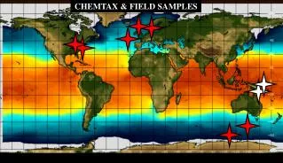
24. Study Area Chlorophyll by satellite

25. Ice shelf 1000m Ice shelf

26. Antarctic Slope Front Pycnocline Tmin

27. ASF Pycnocline Tmin

28. ASF Pycnocline Tmin

29. ASF Pycnocline Tmin

30. ASF Pycnocline Tmin

31. ASF Pycnocline Tmin

32. ASF Pycnocline Tmin

33. ASF Pycnocline Tmin

34. ASF Pycnocline Tmin

35. ASF Pycnocline Tmin

36. BROKE conclusions 1. Effect of Stratification MIXED STRATIFIED Chl a (µg.L-1) 0.4 2.0 Diatoms Pycnocline Pycnocline Prasinophytes Tmin Pycnocline Hapto4s Tmin Pycnocline 2. ‘Hole’ in algal distribution at the ice edge, except for Cryptophytes 3. Generally uniform to pycnocline under ice 4. Importance of frontal features - downwelling tongue from Tmin layer These observations could not have been obtained using microscopy or any other method currently available.

37. Optimizing pigment data

38. Optimising pigment data Aim: Sensitivity – maximum peak height Accuracy Integrity – lack of pigment degradation Reproducibility of retention times Data reliability These aims require care at each step of the process

39. Field sampling It is important to realise that the pigment composition of the sample starts changing from the moment it is enclosed in a dark Niskin bottle. For maximum reproducibility of pigment ratios, all samples should be subjected to the same time delay from collection to end of filtration, and all should be handled in the same light regime (preferably very dim). For example, in our cruises, it is normally 40 minutes before we can sample the Niskin bottles after the physical and chemical oceanographers have collected their samples. Thus we never see diatoxanthin. It has all been converted to diadinoxanthin in the dark.

40. Sample filtration Dim light, cool lab Fluorescence check (each sample is measured in a Turner fluorometer - double checks HPLC result) Small filter (13mm GF/F, extractable in 1.5 ml solvent) Removal of water from filter reproducibly Double label cryotubes (black pen & engraver) Freeze in liq. N2 – directly into 45 L Dewar

41. Extraction Sonication in methanol Small volumes (1.5ml) Internal standard 140 ng β–apo-8’-carotenal (Fluka) Precision Accounts for volume changes Checks injection status Straight to refrigerated (-10°C) autoinjector stage

42. More on the internal standard and data reliability As well as improving analytical precision, the internal standard provides data reliability. Thus if you have a sample with no chlorophyll but a good internal standard peak, then you know that the injection and the chromatogram are OK. The filtration may have been faulty (e.g. holed filter). This is where you go back to check the fluorescence measurement you made while filtering. The fluorescence check has also saved us when fatigued shipboard workers have labelled two sets of cryotubes with the same numbers!

43. A photographic sequence of pigment extraction has been omitted here, to reduce the size of the file. It will be posted on the Australian Antarctic Division web site. The address will be forwarded to the PICODIV site.

44. Our extraction procedure Extraction is performed in 2.5ml plastic syringes, with a leur lock tap. Add 1.5 ml cold methanol Add 25 ul internal standard solution with ~140ng apo-8’-carotenal (Fluka) (add these first to avoid delays once filter is thawed) Remove frozen filter from cryotube While still frozen, cut 1 x lengthways, 4 x sideways into small pieces, with small scissors. Pieces fall into the syringe and thaw. Extract with a probe sonicator (4mm diameter, 50 W, 60 seconds), moving the syringe up and down to ensure that no pieces of filter avoid the sonic beam. The filter is completely disrupted into a slurry. It gets quite warm. Immediately put a plunger into the syringe, attach a 3 mm dia. leur lock filter (0.45 um, nylon, Advantec MFS Inc) and a needle, and squirt the extract into an amber autosampler vial. Place the autosampler vial immediately into a refrigerated (-10°C) autosampler rack. This process averages 1 min 40 sec from starting cutting to completion. All syringe parts are washed with ethanol and dried before reassembly

45. HPLC Analysis Reproducibility Make up solvents by weight Column thermostatted in a water bath (more stable than air oven) Autoinjection Tubing minimum length

46. RT BB carot Chl a Int Std diatox dinox diad peridinin Chl c2 Graph showing reproducibility of retention times through the day for a series of dinoflagellate samples Sample #

47. HPLC Analysis Peak identification Mixed standard every batch RT table Check column performance Reference spectral library

48. HPLC Method (1991): Wright et al., 1991 • The SCOR/UNESCO method • separated 52 pigments in 20 minutes • C18 monomeric column • Ternary gradient • Methanol + ammonium acetate • Acetonitrile • Ethyl acetate • Excellent resolution of marker carotenoids • Inadequate resolution of polar chlorophylls and divinyl chlorophylls

49. HPLC Method (2000): Zapata et al. (2000) • Waters Symmetry C8 (monomeric) column • Binary gradient • A=Methanol:acetonitrile:pyridine (pH 5.0) (50:25:25 v/v/v) • B= Methanol:acetonitrile:acetone (20:60:20 v/v/v) • 25C • Main technique in our lab • Good resolution of marker carotenoids, esp fucoxanthin derivs • Excellent resolution of polar chlorophylls • Divinyl chlorophylls resolved from chlorophylls • Resolution order differs from Wright et al. (1991) • Complementary techniques

50. Peak detection Diode array detection 436 nm 470 nm 665 nm 400 – 480 nm (sum) (summing the wavelengths on the diode array detector provides about 3 x improvement in signal : noise ratio This greatly improves sensitivity) Fluorescence detection excitation: Broad band blue (Turner fluorometer filter) emission: Long pass red (> 630nm)