Download
1 / 1
10 likes | 110 Vues
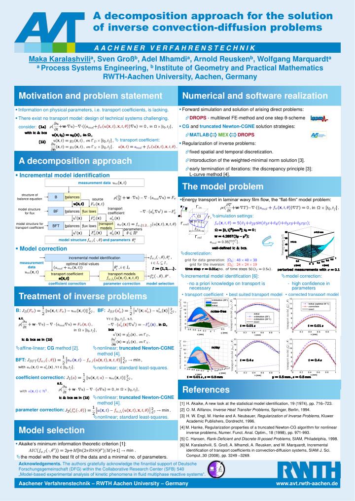
A decomposition approach for the solution of inverse convection-diffusion problems. Motivation and problem statement. Numerical and software realization. Forward simulation and solution of arising direct problems: DROPS - multilevel FE-method and o ne step θ-scheme

E N D
A decomposition approach for the solution of inverse convection-diffusion problems Motivation and problem statement Numerical and software realization • Forward simulation and solution of arising direct problems: • DROPS-multilevel FE-method and one step θ-scheme • CG and truncatedNewton-CGNE solution strategies: • MATLABMEXDROPS • Regularization of inverse problems: • fixed spatial and temporal discretization. • intoroduction of the weighted-minimal norm solution [3]. • early termination of iterations: the discrepancy principle [3]; L-curve method [4]. • Information on physical parameters, i.e. transport coefficients, is lacking. • There exist no transport model: design of technical systems challenging. consider: • transport coefficient: A decomposition approach • Incremental model identification The model problem measurement data structure of balance equation B balances • Energy transport in laminar wavy film flow, the “flat-film“ model problem: source transport coefficient model structure for flux BF balances flux laws • simulation settings: model structure for transport coefficient BFT balances flux laws transport models parameters model structure and parameters • Model correction • discretization: incremental model identification measurement data optimal initial values transport coefficient transport models • incremental model identification [6]: • no a priori knowledge on transport is necessary • model correction: • high confidence in parameters coefficient correction parameter correction model selection Treatment of inverse problems • transport coefficient • best suited transport model • corrected transport model B: BF: • affine-linear; CG method [2]. • nonlinear; truncatedNewton-CGNE method[4]. BFT: • nonlinear; standard least-squares. coefficient correction: References • nonlinear; truncatedNewton-CGNE method[4]. [1] H. Akaike, A new look at the statistical model identification, 19 (1974), pp. 716–723. [2] O. M. Alifanov, Inverse Heat Transfer Problems, Springer, Berlin, 1994. [3] H. W. Engl, M. Hanke and A. Neubauer, Regularization of Inverse Problems, Kluwer Academic Publishers, Dordrecht, 1996. [4] M. Hanke, Regularization properties of a truncated Newton-CG algorithm for nonlinear inverse problems, Numer. Funct. Anal. Optim., 18 (1998), pp. 971-993. [5] C. Hansen, Rank-Deficient and Discrete Ill-posed Problems, SIAM, Philadelphia, 1998. [6] M. Karalashvili, S. Groß, A. Mhamdi, A. Reusken, and W. Marquardt, Incremental identification of transport coefficients in convection-diffusion systems, SIAM J. Sci. Comput.,30 (2008), pp. 3249 –3269. parameter correction: • nonlinear; standard least-squares. Model selection • Akaike‘s minimum information theoretic criterion [1]: • the model with the best fit of the data and a minimal no. of parameters.