Download
1 / 49
500 likes | 610 Vues
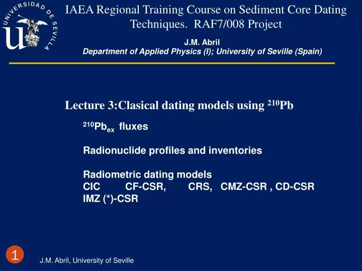
IAEA Regional Training Course on Sediment Core Dating Techniques. RAF7/008 Project. J.M. Abril Department of Applied Physics (I); University of Seville (Spain). Lecture 3:Clasical dating models using 210 Pb 210 Pb ex fluxes Radionuclide profiles and inventories Radiometric dating models

E N D
IAEA Regional Training Course on Sediment Core Dating Techniques. RAF7/008 Project J.M. Abril Department of Applied Physics (I); University of Seville (Spain) • Lecture 3:Clasical dating models using 210Pb • 210Pbex fluxes • Radionuclide profiles and inventories • Radiometric dating models • CIC CF-CSR, CRS, CMZ-CSR , CD-CSR • IMZ (*)-CSR J.M. Abril, University of Seville
2 J.M. Abril, University of Seville
aw z 137Cs 222Rn 210Pb J.M. Abril, University of Seville
222Rn exhalation depends, among other factors, on 226Ra content in soil, soil texture and structure, water content, and the forcing factors… Abril et al. (JENVRAD, 2009) 4 J.M. Abril, University of Seville
J.M. Abril, University of Seville Author: Israel López, Univ. Huelva (Spain)
Some global patterns for 210Pbex fallout • Predominant west-east movement of air masses 210Pbex fallout is low in the western areas of the continents • 210Pbex fallout is higher in the North hemisphere • 210Pbex fallout is positively correlated with rainfall Figures from P.G. Appleby, STUK-A145 J.M. Abril, University of Seville
Some reference values for annual fallout of excess 210Pb (Bq m-2 y-1) Global scale , F ~ 23-367 Bq m-2 y-1 (Robbins, 1978) Tropical Australia , F ~ 50 Bq m-2 y-1 (Brunskill and Pfitzner,2000) Inputs and Inventories (Bq m-2 ) in sediments Catchment concentration factor (normalization or focusing factor) : Z Input (*) = ZF Steady State Inventories Σ = ZF/λ For 210Pb = ln2/T1/2 with T1/2 = 22.26 y. J.M. Abril, University of Seville
210Pb [Bq/kg] total 210Pb (unsupported) 226Ra Z [cm] Radiometric dating with 210Pb: Basic aspects Supported fraction If we assume that there is no Rn exhalation from the sediment, then the total activity of 210Pbtotal will be 210Pbtotal = 210Pbsupported + 210Pbunsupported and 210Pbsupported = 226Ra activity J.M. Abril, University of Seville
aw z Basic Concepts and definitions J.M. Abril, University of Seville
V mw ms z Bulk density Compaction and bulk density As depth increases in the sediment core, water pores are replaced by solids Saturated porous media J.M. Abril, University of Seville
mw m w ms s Drying and gravimetric method Practical measurement of bulk densities J.M. Abril, University of Seville
Practical measurement of bulk densities. Refinement mw w m ms,o s,0 ms,i s,i Drying and gravimetric method and loss by ignition J.M. Abril, University of Seville
0.7 0.6 0.5 0.4 (g/cm3) 0.3 0.2 0.1 0 0 5 10 15 20 Depth [cm] Bulk density versus depth profiles in sediment cores J.M. Abril, University of Seville
[ g dry weight cm-2] z Mass thickness, Δm , and mass depth:, m Δz J.M. Abril, University of Seville
[ g dry weight cm-2 y-1] (Mass) Sedimentation rate : w ≈ A (Zi-1, t) w (Zi-1, t) Time versus m for constant w (*) A (Zi, t) Zi w (Zi+1, t) A (Zi+1, t) Z J.M. Abril, University of Seville
Basic processes ≈ A (Zi-1, t) w (Zi-1, t) A (Zi, t) Zi w (Zi+1, t) A (Zi+1, t) Z J.M. Abril, University of Seville
Fundamental equations Mass conservation for a particle-associated radiotracer Mass conservation for solids BOUNDARY CONDITIONS In situations where the tracer is partially carried by pore water or in presence of selective and/or translocational bioturbation Eqs. has to be revisited J.M. Abril, University of Seville
Constant Flux and Constant Sedimentation rate (CF-CSR) F incoming flux [Bq L-2 T-1] w sedimentation rate Activity concentration at interface (non post-depositional mixing) Constant A0 J.M. Abril, University of Seville
The sediment-water interface displaces upwards z=z(t) Specific activity A0 Layer at time t=0 time = 0 time = t =m/w m=m(t) (non post-depositional mixing) J.M. Abril, University of Seville
Ln(A) m Curve-fitting model , free parameters : Ao , w Validation: Goldberg first validated the 210Pb dating method in varved sediments Think about: Any implicit assumption concerning compaction? J.M. Abril, University of Seville
EXAMPLE from a case study ZF = 172 Bq m-2 y-1 J.M. Abril, University of Seville
w , (mass) sedimentation rate Dates or chronology: Year of sampling – Age Age : T(m) or T(z) , from m(z)/w Don't forget: Estimated sedimentation rates, ages and dates have to be provided with the corresponding uncertainties. W = 0.115 ± 0.014 g cm-2 y-1 J.M. Abril, University of Seville
Associated uncertainties in 210Pb chronology General formulae for error propagation m G.F. J.M. Abril, University of Seville
w Lest squares fitting a, b, R2 easily produced with excel or other shifts Associated uncertainties in 210Pb chronology t J.M. Abril, University of Seville
Time resolution . Each sectioned layer in the core corresponds to a time interval Δt = dm/w Remember: As the analytical method is homogenizing the material from each layer, it is not possible to solve other time marks within such an interval (e.g. two 137-Cs peaks). • Note for advanced students: • Apply lineal regression taking into account the associated uncertainties in measurements J.M. Abril, University of Seville
CAUTION ! • Estimation of the supported fraction is not a trivial task ! • 226Ra may be non uniform in depth and being different from the 210Pb baseline • Settling particles can be depleted in 226Ra in the water column while enriched in 210Pb Data fromAxelsson and El-Daoushy, 1989 J.M. Abril, University of Seville
10000 Redó Gossenkollesee 1000 210Pb (Bq/kg) 100 10 0 0.2 0.4 0.6 0.8 1 Mass depth (g cm-2) PROBLEMS: 1.- Many unsupported 210Pb profiles do not follow a simple exponential decay pattern More complex models are required J.M. Abril, University of Seville
CIC model (Constant Initial Concentration) F incoming flux sedimentation rate w Activity concentration at interface (no post-depositional mixing) • CIC modelassumes constant Ao; Thus, changes in F must be compensated with changes in w. • Also , it assumes non post-depositional mixing • Reasonable when F is associated with inputs of solids J.M. Abril, University of Seville
CIC model can equally be formulated in terms of actual depth (z) or mass depth (m) A A0 A(m) Chronology (one date per data point) m Alternative estimation of sedimentation rates (one per data point) – only for cores with high spatial resolution- • Unknowns for CIC: Ao and wi (N+1; N= number of sections in the core) • It is a “mapping” model • CAUTION ! • Estimation of the initial concentration, Ao, is not a trivial task ! J.M. Abril, University of Seville
EXAMPLE from a case study ZF (recent) = 76 Bq m-2 y-1 CF-CSR CIC J.M. Abril, University of Seville
CRS model (Constant Rate of Supply) F incoming flux w Initial concentration CRS modelassumes constant F, independently of w. Ao can vary. Also assumes non post-depositional mixing. -Reasonable when F is not coupled with inputs of matter J.M. Abril, University of Seville
After a time t, the horizon now at z=0 will be located at depth z(t), and because of the radioactive decay. At “geological” timescale the inventory is steady state; thus, CRS model Inventory under the horizon z z Z J.M. Abril, University of Seville
Once the chronology is established, sedimentation rates can be obtained for each two adjacent layers: CRS model CRS Chronology: Alternatively, from the mass balance in the steady state inventory below depth z z • Unknowns for CRS: F, wi (N+1; N= number of sections in the core) • It is a “mapping” model J.M. Abril, University of Seville
CAUTION • Check for completeness of inventories (sometimes it will be necessary to estimate the “missing” part of the total inventory) J.M. Abril, University of Seville
EXAMPLE from a case study J.M. Abril, University of Seville
ZF = 170 Bq m-2 y-1 from CF-CSR w = 0.115 ± 0.014 g cm-2 y-1 J.M. Abril, University of Seville
Steady-state mass balance F Aama Radioactive decay wAa Sediment growth Complete mixing zone model with constant sedimentation rate and constant flux. F w ma Mixing Curve-fitting model , free parameters : Aa, w, ma J.M. Abril, University of Seville
Example CMZ-1 mixing ma=9.5 g cm-2; w=0,374 g cm-2 y-1 J.M. Abril, University of Seville
10000 Redó Gossenkollesee 1000 210Pb (Bq/kg) 100 10 0 0.2 0.4 0.6 0.8 1 Mass depth (g cm-2) PROBLEMS: 2.- Many times unsupported 210Pb profiles can be equally explained by different models 210Pb chronologies must be validated against an independent dating method Acceleration or mixing? J.M. Abril, University of Seville
Think about: What other hypothesis are implicitly assumed in all the previous models ? J.M. Abril, University of Seville
Constant flux, CSR and constant difussion Model Demonstration will be provided within lecture 6 Curve-fitting model , free parameters : ZF, km , w Data: CF-CS-C Diffusion Fit : CF-CSR Model J.M. Abril, University of Seville
J. N. Smith proposed a protocol for research journals for the acceptance of papers that rely on 210Pb dating to establish a sediment core geochronology: ‘‘The 210Pb geochronology must be validated using at least one independent tracer which separately provides an unambiguous time-stratigraphic horizon’’. J.M. Abril, University of Seville
Examples generated with numerical solutions Constat aceleration, constant diffusion or CF-CSR? ZFo=10 mBq/(cm^2 y) , w=0.1+0.1 t/150 g/(cm^2 y) D=0 J.M. Abril, University of Seville
Examples generated with numerical solutions Effect of “episodic” changes in sedimentation rates? J.M. Abril, University of Seville
λ=0 Ts =150 y T= - 50 y sgt= 5 y Numerical algorithm: MSOU J.M. Abril, University of Seville
λ=0 Ts =150 y T= - 20 y sgt= 2 y Numerical algorithm: MSOU J.M. Abril, University of Seville
Examples generated with numerical solutions When data are smooth enough to apply CSR models? Periodic changes in w with T=7 y J.M. Abril, University of Seville