Download
1 / 53
540 likes | 1.06k Vues
Sine waves and Decibels. Southern Methodist University EETS7320 Fall 2007 Lecture 3 Slides only. (No notes.). PSTN Transmission Technology in 1960. Analog transmission of voice channel signals

E N D
Sine waves and Decibels Southern Methodist University EETS7320 Fall 2007 Lecture 3 Slides only. (No notes.)
PSTN Transmission Technology in 1960 • Analog transmission of voice channel signals • Analog amplifiers (“repeaters”) inserted in long transmission lines compensate for primarily resistive losses • Analog frequency division multiplexer (FDM) used for long distance • Shortcomings of analog amplifiers, even with the use of “negative feedback”: • Some distortion “peak flattening” of waveforms • Some random noise added by each amplifier • Transistors (vis-à-vis vacuum tubes) slightly extended the useful life of analog technology • From 1960 to today (2005) digital multiplexing transmission technology has almost completely replaced analog transmission • Widespread rapid growth of digital multiplexing (e.g. T-1 or E-1) facilitated the introduction of digital switching
PSTN Switching Technology in 1960 • Dial-up calls switched via electromechanical “space-division” switches • Old Strowger step-by-step “(“gross motion”) switches • Newer “crossbar” (“fine motion”) electromechanical switches. Intended evolution of switching until eventually superseded by digital switching • Then new computer controlled analog switches (example AT&T 1ESS – electronic switching system) • Quite sophisticated control and call processing • Switching used small “reed relay” metallic contacts • From 1960 to today (2005) digital switching has almost totally replaced analog
Data Communication in 1960 • Modulator-demodulators (MODEMs) using frequency-shift-keying (FSK) modulation were in limited use via dial-up PSTN connections • Data rates up to 110 bit/second typically used with electromechanical “teletypewriter exchange” (TWX) services via voice channels. • TWX was an AT&T competitor to the Western Union TELEX service. Telex used special electromechanical switches and a separate private network. TWX and Telex have since been substantially supplanted by Internet e-mail. • Higher modem bit rates (<2400 bits/second) typically required a leased point-to-point line with a fixed “equalizer” (analog waveform compensation to correct for waveform changes due to transmission impairments) • Costly and slow-response installation requiring skilled technicians • Self-adaptive equalizers opened the dial-up market to higher bit rate data transmission for computers, etc.
Legacy Methods and Jargon • The subscriber loop and telephone set still use analog waveforms in the vast majority of installations today • Speech or test waveform power level is described using decibels (dB) • Proportional to common logarithm of the ratio of the power compared to a 1 milliwatt (mW) reference signal • Historically introduced about 1910. One dB described the input-output power ratio of a 1 kHz test tone in a mile (1.6km) of 19 ga copper wire*. • Calculation of total “loss” (output power/ input power) for cascaded transmission equipment (e.g., several miles of wire) requires adding dB values, rather than multiplying power ratios. • Unlike a MODEM, the human ear is not sensitive to waveform changes caused by varying delay of different frequency components of a waveform. Therefore, measurement of signal power vs. test sine wave frequency is sufficient to characterize an analog telephone channel. *North American wire gauge units (ga or AWG) explained later.
Sine Wave Test Signals • Analog telephone channels, and end-to-end performance of analog channels with a digitally coded transmission segment in the middle, can be characterized via: • Signal power output-input ratio (expressed in dB) vs. frequency (Hz), using a sine wave test signal • For example, power loss must be uniform within limits stated in ITU standards over the frequency range 300 Hz to 3500 Hz. • For MODEM use, the test signal time delay vs. frequency • Alternatively to time delay: phase shift vs. frequency. • Above information typically described via a two-axis graph or a table (list) • Any non-sinusoidal waveform can theoretically be made up of a sum of various properly chosen sine waves of different amplitudes and frequencies. • So-called “Fourier analysis and synthesis” • Analysis of arbitrary waveform results can be theoretically computed with relative ease
Example Voice Channel Power v. Frequency Graph dB This is derived from the amplitude vs. frequency Measurement. 0 -3 -3 dB (“half power”) point is used only because it is convenient for measurements. 300 Hz low frequency signal drop off is result of coupling transformers in the subscriber line circuit. 3500 Hz high frequency signal drop off is result of intentional low pass filter design, to retain adequate signal quality for a conversation. -10 -20 -30 kHz 0 1 2 3 3500 4 300
Describing Linear Systems • Many telecommunications transmission system elements are accurately described by linear equations. • Example linear equation: y= K•x, where y and x are measurable system variables like voltage and current and K is a constant. • Another example: y= K•(dx/dt), showing that a time derivative is a linear “operation” • Many electrical devices like resistors, capacitors, inductors and transmission lines (wire, cable) are inherently linear. • Some devices, like amplifiers, are non-linear overall, but are intentionally designed and used in only a part of their range of voltage and current where they appear to be linear.
Graphical Representations y v (0,0) x i vout vo Linear range vin vi
Linear System Analysis • Linear devices and systems can be described for purposes of analysis or design, by either of two methods: • Time domain analysis: output waveform, described as graph/table/list of voltage vs. time, in response to ideal impulse input • Frequency domain analysis: two graphs/tables/lists showing amplitude vs. frequency and phase (time delay) vs. frequency) in response to input sine wave at many test frequencies
Ideal Unit Impulse Symbolic: pulse time very small, Pulse voltage very big. v•s v 1 t t • The unit impulse is a theoretical waveform that is zero amplitude for all time before and after time t=0. • At time t=0, it is “infinitely” large, so that its “area’ when drawn on a graph is unity (1). • For the case where the impulse is a voltage, its “area” is stated as one volt-second. When the impulse is a fluid flow quantity like liters/second, its “area” is stated as one liter. • Symbols used for this waveform are: u0(t) or (t) or I(t). • The time integral of a unit impulse is a unit step. • For real-life measurement of the impulse response, measure or “capture” the step response, then compute the time derivative of the step response. This derivative waveform, treated as a voltage waveform is the impulse response. Note: A volt-second is also called a weber (Wb).
Time Domain Analysis Example v input output Impulse response System To compute output for an arbitrary input, cut input waveform into small pieces and replace each piece with an impulse of equal area. Each input impulse produces a proportional and delayed impulse response. Add all of these. A formal method to do this is called the convolution integral (calculus). t v v input t t v Approximate output waveform made up of sum of several copies of the impulse response (delayed and scaled to the input signal). For theoretical analysis we find the result of infinitely many very closely spaced impulse responses. t
Frequency Domain Analysis • Using a sine wave generator of unit amplitude, feed a sine waveform into the system at every frequency. Theoretically this requires an infinite number of distinct frequency choices. • For each input sine wave (actually a cosine wave) frequency, the output will also be a sine wave having the same frequency but in general a different amplitude and phase (time delay) relative to the input sine wave. • This information is compiled into two lists, amplitude vs. frequency and phase vs. frequency. • When an input waveform is already properly described by means of a similar pair of lists, compute the frequency domain description of the output by means of these operations: • The amplitude of the output signal is the product (multiply) of the input amplitude and the system amplitude. • The phase of the output signal is the sum (add) of the phase of the input and the phase of the system.
Comparison • The multiplication (of amplitudes) and addition (of phases) used in frequency domain analysis are simpler than the use of integral calculus to compute the convolution integral in time domain analysis. • But we ultimately live in the time domain, so to determine the output waveform somebody somehow somewhere must do some integral calculus. • Books are available containing tables of “transforms” listing the frequency domain description (via table,list, graph or formula) for many well-know time domain waveforms.
Time-Frequency Domain Relationships • The two methods are theoretically related • The unit impulse waveform can be shown to be equal to the sum of infinitely many cosine waves (each of unit amplitude). • In general, each time domain input waveform can be “transformed” (described in the form of a frequency domain list/table/formula). The frequency domain data for many well-known waveforms (step, triangular waveforms, etc.) are given in mathematical handbooks and treatises, or they can be computed by means of well-known methods or via numerical calculation using digital computers. • This process of converting from a waveform in time domain to a description in the frequency domain is called a Fourier transform, after its inventor. • A similar process, called LaPlace transformation, is not described here. Note: Fourier (a French name) is pronounced /four-yay/
Why Engineers Love Sine Waves* • Linear systems can be analyzed relatively simply for sine wave signals using complex number algebra • Differential/integral equations are not needed explicitly • Sine waves and “real” exponential waveforms are “natural behavior” waveforms of linear systems • The natural oscillations of linear time-invariant electrical (and mechanical) systems comprise • Sine/cosine waves • “Real” exponential waveforms • Product combinations of these two • Many systems are designed to use sine waves partly because of ease of analysis: • Electric power systems use 50 Hz or 60 Hz sine waves (400Hz on aircraft). • Originally, electrically linear devices like incandescent lights, motors, etc. were the only devices in power networks. Today we get harmonic power waveform distortion from fluorescent lights and other non-linear electronic equipment! • Radio broadcasting carrier waveforms * Many engineers also have passionate feelings for electrons, as well!
More Sine Wave Features • Fourier Series: Any periodic (cyclic repetitive) waveform can be mathematically expressed as a discrete sum of (possibly an infinite series of) sine waves. • The base frequency of the series of sine waves is the same as the repetition frequency of the waveform to be described • The waveform can have step discontinuities in voltage, sharp impulses, other bizarre mathematical features… • Fourier Integral: Any non-repetitive waveform can be mathematically expressed as an integral (summation of an uncountable continuum) of sine waves at all frequencies. • Again discontinuous and impulsive waveforms are allowable • Distinct radio transmissions are separated from each other by means of a transmitter and receiver that purposely produce a radio waveform of limited sinusoidal waveform bandwidth and a receiver that amplifies and processes (detects) only a corresponding limited portion of the radio frequency sine wave spectrum.
Natural Waveforms of Linear Systems • Sine wave • Exponential • Product of the two Both waveforms are subsets of the class of complex exponential mathematical functions.
What is a Linear System? • Consider physical systems having “input” and “output” waveforms • Waveforms may be current, voltage, mechanical variables like velocity, current, force, etc. [v(t), i(t), f(t), etc.] • Each input waveform produces a distinct output waveform • Consider a compound input waveform made up of the sum of two other waveforms • In a linear system, the “output” due to such a compound “input” is the sum of the outputs due to each input acting alone • Sometimes called the “principle of superposition” • Note: Do not confuse this technological jargon meaning of “linear” with the currently popular alternative meaning of “sequential” or “consecutive”
Properties of Linear Systems • Multiplying the input amplitude by a constant number factor m causes the output to increase in amplitude by the same factor m • If input waveform f(t) produces output waveform g(t), then higher amplitude waveform m•f(t) produces higher amplitude output waveform m•g(t) • A system described by linear algebraic equations with constant coefficients is a time-invariant linear system: z = A•x + B•y w= C•x + D•y If A,B,C, D are not constants, but vary with time, but do not depend on w,x,y or z, the system is still linear, but not with constant coefficients . Linear time-varying systems still follow the principle of superposition, but their “natural” behavior waveforms may not be sine waves • A system accurately described by linear differential or integral equations is also linear: example, a capacitor: i = C•dv/dt
Many Actual Systems are Intended to be Linear • Electric circuits consisting of resistors, capacitors, inductors, transformers and transmission lines are linear when used within their design range • However, inductors and transformers can be “over driven” into a non-linear regions of current due to non-linear magnetic properties of some materials, like iron (careful!) • If resistors get hot enough to burn or melt, they no longer have “constant coefficients” of resistance • Most electronic devices like diodes, transistors, etc., are very non-linear • When “small signals” (low amplitude) are used, their properties are approximately linear • Many electronic systems which are not precisely linear can be approximately described as linear over a restricted range of voltage or current.
A Sine Wave • The “shadow” or projection onto one axis, of a point moving in a circle in 2-dimensional space • Here, f1 is 1 Hz, amplitude is 1, period is 1 second, initial phase angle is zero.
Three Sine Wave Properties • Frequency • common unit: cycles per second or hertz (Hz) • Other units: degrees per second, radians per second, etc. (360 degrees or 2• = 6.28... radians in one cycle or turn) • Period or cycle duration is the reciprocal of frequency: T=1/f • Amplitude • Unit: the physical quantity which the sine wave represents; amperes (current), volts (voltage), etc. • Phase (angle) or time delay • relative delay or time offset compared to a reference waveform or clock signal • Unit: expressed in degrees, radians, fractions of a cycle, or in time units (seconds, etc.)
Example Non-smooth appearance of sine wave is an artifact of the drawing software. amplitude frequency phase Peak amplitude 2.7 volts (corresponds to 1.909 v RMS • phase delay compared to cosine wave reference is /8 radians, or 22.5º or 1/16 cycle, or 0.0125 sec or 12.5 milliseconds period or interval is 0.2 sec, or 200 milliseconds. Then frequency is 1/(0.2) or 5 Hz. Note: Sine wave with 90º phase advance is equivalent to a Cosine wave.
Sine Waves in Linear Systems • Sine wave input to a linear time invariant system produces sine wave output (in “sinusoidal steady state”) • In many cases there is also a “transient” or start-up response (decreasing exponential) waveform which eventually “dies out” (amplitude becomes very small). • Output is precisely the same frequency as the input • The only output parameters that can differ from the input waveform are: • Physical value (current vs. voltage, for example) • Amplitude • Phase • The amplitude and phase may be expressed symbolically in complex number algebra (real and imaginary numbers) by one two-part symbol on paper. • “Real” ratios such as resistance (ohm=volt/amp) can be generalized to a complex number called “impedance” which indicates both the magnitude ratio and the phase angle difference as well.
Why is Linearity Important? • Non-linear systems, in general, produce signals which have different sinusoidal frequency waveforms at the output than the sine wave frequency used at the input • Some systems exploit this property -- radio receivers incorporate a “down converter” which produces internal radio signals at a lower frequency than the radio input waveform at the antenna. Lower frequency waveforms are often less complicated to process and equipment is thus less costly. • One such radio process: “detection” or “demodulation” -- extracts original information waveform such as speech or digital information. • When other undesired frequencies are produced, this is called Inter-Modulation (IM) • When it occurs just as desired, it is called Modulation. This usually involves intentionally generating a waveform which is the instantaneous arithmetic product of two waveforms. • The word “modulation” has several meanings, some rather vague.
Ultra Wide Band • The only propose radio signal competitor to using a modulated sine wave is UWB, which proposes to use approximately periodic extremely brief high amplitude electromagnetic pulses • Information is conveyed by varying the time interval between the pulses • This is sometimes called “pulse position modulation” PPM • Proponents claim that the large rf bandwidth and the low amount of UWB power in a typical narrower signal bandwidth permits simultaneous operation without mutual interference • Some opponents dispute such claims in fundamentals • Other opponents assert that the inter-modulation of UWB and other ordinary bandwidth signals is inherently severe, and causes serious interference to ordinary bandwidth signals. • At this time, efforts are still underway to utilize UWB, and not all parties agree.
“Modulation” of a Square Wave Fig. 1 PWM • A square wave (in contrast to a sine wave) is seldom modulated in either frequency or amplitude in modern electronics, although that is technologically feasible. • Some equipment “modulates” the width of square pulses (PWM). See Fig. 1 • Some equipment modulates the position of a pulse in the time window T reserved for each period of pulse transmission (PPM). Fig. 2. One type of PPM is “ultra-wide-band” radio. • Incidentally, PPM waveform is the approximate time derivative of a corresponding PWM waveform. • We speak of “pulse code modulation” (PCM) where an analog voltage is measured and the measured voltage is encoded as a sequence of binary pulses (amplitude either 5 volts or zero volts). PCM is unlike PWM or PPM. T Fig. 2 PPM time
Sine Waves, Signals, and Spectrum Analysis Any waveform may be theoretically described as a combination of sine and cosine waves of various frequencies: • Fourier series for periodic waveforms • Frequencies are integral multiples of basic repetition frequency • Fourier integral for non-periodic waveforms • Theoretically infinite number of frequency components • Other mathematical descriptions are used for special purposes, as well: • Power* series: y = ao + a1•t + a2•t2 + a3•t3 … is used in linear predictive speech coders, for example. • Power series coefficients ao,a1,etc. derived from nth time derivative of waveform to be described... *Also called Taylor or MacLaurin Series.
Linear systems are described two ways: • Response to sine waves of (theoretically) all frequencies • List(s), graph(s)or other descriptions are used • Describe amplitude and phase of output for each frequency • Test input is a unit amplitude cosine wave (sine wave with 90º phase advance) at each test frequency • Impulse response (time domain) • Output is a waveform produced by a theoretical input pulse signal • Input, in theory, is an instantaneous impulse of infinite amplitude and unit “area” (in volt•sec, for example) • For practical lab measurements on systems having a limited linear range of operation, a unit step input voltage is used. The time deerivative of the output is the impulse response. • These two descriptions are theoretically mutually derivable, either one from the other
Sample Circuit with Resistors and Capacitors Adjustable Frequency Sine-wave Test Signal Generator + V1 -- + V2 -- Voltage-ratio meter, with display showing ratio as a function of oscillatory frequency.
What to Display and Why... • Computing, tabulating or plotting a graph of the ratio of output/input voltage allows us to compute the absolute output voltage for any specific input voltage waveform. • Logarithmic graph axis displays a wide range of frequency (or voltage or power). • In certain types of electric devices, the slope of some asymptotic lines (log voltage vs. log frequency) is exactly 1, 2, etc., indicating that voltage is proportional to the frequency, the square of the frequency, etc. • The unit scale is normally chosen so the labeled axes are integral values such as 1, 2, 5, 10, 20, 50, 100 etc. The peculiar numbers in the following examples are an artifact of the graphics software, which needs to be improved!! • Two times the log of the voltage ratio shows the power ratio (in systems having the same ratio of voltage to current at input and output). Twenty times the log of the voltage ratio in such a case is called the decibel (dB) power ratio.
Logarithms • 18th century Scottish mathematician Napier noted that when multiplying two numbers that were expressed as powers of the same base, the exponents were simply added. When dividing, the exponent of the divisor is subtracted. Examples (using base 2): • 32•16= 25• 24= 2(5+4) = 29 = 512 • 512/128 = 29/27 = 2(9-7) = 22 = 4 • Napier computed and published a table of base-10 (so-called “common”) logarithms to reduce the labor required for multiplying and dividing. • Logarithms were extensively taught in schools before the availability of electronic calculators. They have many other mathematical uses as well. • Logarithms are the basis of the “slide rule” which has also been substantially supplanted by the electronic calculator or computer.
Amplitude Ratio (V2/V1) Graph Peak amplitude ~ 0.62 “Half-power” amplitude 0.44:= 0.62•0.707 Bandwidth Based on Half-power points
Significance of These Graphs • The previous graphs show that a simple electric circuit using capacitors and resistors can perform the operation of frequency “filtering” (not the best filter example, but simple to analyze) • In this example, the output voltage (or power) is maximum for a frequency of about 35 Hz. • The output voltage is much lower (“more attenuated”) for higher or lower frequencies. • The output voltage is very small (in fact, zero although the logarithmic axes do not show this) for zero frequency and “infinite” frequency. • Such a “band pass” filter is used to separate one radio frequency from others so a radio receiver can receive a desired broadcast or cellular conversation. • Most band pass filters used in radio use inductor components (in addition to resistors and capacitors) to achieve sharper or more narrow peaks of output vs. frequency (improved selectivity). Electro-acoustic (quartz crystal) and other filter devices are also used. • Other circuit configurations may be used to produce “high pass” and “low pass” filters. • Low pass filters are used to attenuate the higher audio frequency components of a voice waveform before digital sampling and coding.
Radio Tuning Filter Example ~ ~ Bandwidth at half Power points is R/(4•p•L). 70.7% voltage point is the 50% power point. C |V/I| ~ + V - R L I • Filter circuit using both inductors and capacitors produces a “sharper” peak response than resistor-capacitor filters • It can “filter” one desired radio frequency waveform out of many different frequencies (attenuates other frequency ranges) • Small R value implies very narrow bandwidth, good “selectivity” • Filter center frequency fo is modified by mechanically adjustable capacitor value C in older radios. • Newer radio receivers have a fixed fo center frequency, and a variable frequency (“local”) oscillator. A replica of the desired radio frequency is produced via an interaction between the desired frequency waveform and the local oscillator waveform in a non-linear circuit. This device is called a frequency-adjustable down-convertor. f “Band-pass” Graphic Filter Symbol fo=1/(2•p•L•C)
Illustrating Fourier* Series • The following pages illustrate how a square wave can be approximated by adding several sine waves of appropriate frequencies and amplitudes. These frequencies must be each an exact integral multiple of the frequency of the square wave signal to be approximated • The coefficients can be computed by Fourier analysis • The coefficient for the nth term is proportional to the area (integral) of the product waveform of the square wave and the particular sine wave at that frequency • For a square wave, only the 1,3,5,… odd “harmonic” frequencies have non-zero coefficients. *Invented by Joseph B.J.Fourier (pronounced: four-yay), 19th c. French mathematician and explorer.
Approx. Square Wave Using 3 Odd Harmonics Proper amplitude of each “harmonic” sine wave was found from a product integral formula (same as statistical cross correlation).
How Approximate?- I • First, the computer software program* used to produce these graphs is prone to some errors of interpolation • Only 100 data points are plotted for each graph • The waveforms have spurious wiggles which are artifacts of the software • Second, when only a limited number of harmonics are used, there is a “bump” or overshoot peak at each corner of the waveform • Called “Gibbs’ Phenomena” (J.W.Gibbs, 19th c. American Mathematician) • Width of Gibbs’ bumps approaches zero as number of additive terms increases * Mathcad 4.0
How Approximate?- II • “Rise time” of steep slope at corners is faster (shorter rise time) when more high frequency harmonics are included in the Fourier series • We loosely describe any waveform with sharp corners and brief rise time as having “large bandwidth” • Conversely, when we remove high frequency components from a waveform via filtering devices, we: • reduce the bandwidth (reduce the power of the high frequency components of a base band waveform) • increase the rise time of waveform “corners” • change the waveform to some extent • One objective of “high fidelity” is to retain (not remove) the high frequency power from music or speech
Comments on Examples • These square waves use only sine components (no cosines) because they are “odd parity” symmetric about t=0 point. Even-symmetric waveforms use only cosines. General non-symmetric waveforms use both. • Square waves have only odd harmonics (1,3,5…) because they have no “wiggles” that repeat 2, 4, 6… times in a cycle. • General waveforms of arbitrary shape have both odd and even harmonics, sine and cosine components.
“Musical” Analysis • Some* electronic musical instruments, like the original Hammond Organ, produce complicated waveforms by combining higher frequency sine waves of “harmonic” frequencies for each key on the musical keyboard. • These instruments use variable resistors to adjust the coefficients of each “harmonic” component. The phase is not adjustable. Phase adjustment is not needed for music, for reasons to be described. • Some combinations of harmonics are preset to approximate desired sounds like “clarinet,” “trumpet,” etc. • Considering middle C (approx. 260 Hz**) as the fundamental frequency, the first few “harmonics” are: • If we “shift” all of these into the same octave, the result is a major triad chord (C, E, G, C)! *Other modern music synthesizers store the music time waveform using digital samples, similar to the samples in a digital telephone system. *More precisely, middle C is 261.1725 Hz in modern even-tempered concert pitch intonation (with A=440 Hz exactly).
“Peak Clipping” makes all waveforms “square-ish” • A periodic waveform that is modified by a non-linear system so that the positive and negative peaks of each cycle are clipped or flattened, will have a waveform somewhat like a square wave • The square wave comprises numerous odd harmonic sine wave components • One method for quantitatively describing the amount of distortion in “high fidelity” amplifiers is to measure the amount of undesired 3rd harmonic frequency power when a “pure” sine wave is used as input. • This is expressed as a logarithmic power ratio (in decibels) compared to the fundamental frequency signal power. • This is only one example of how a non-linear system produces outputs at different sine wave frequencies than the input frequency
More Fun with Fourier Analysis Other aspects: • Certain analysis and design processes, done mentally or with paper and pencil, are much simpler and faster to do using sine wave components and Fourier analysis. This was particularly significant before the days of widely available computers. • Time derivative and time integral of a waveform can be computed readily from the Fourier series or transform, by multiplication or division by the frequency value (where j represents the “imaginary” square root of negative 1, also called “i” in math and physics documents) (d/dt) h(t) <---> j2fH(f) h(t)dt<---> H(f) / (j2f) • Waveform filtering to remove undesired frequency components • Analysis of speech and other waveforms for efficient coding • Discrete Cosine Transforms for image analysis and coding • Function to be analyzed into component sine waves is a graph of color brightness as a function of x-axis distance measured across the picture or image
Partial Spectrum Information is Adequate for Voice Signals • In general, we need both amplitude and phase (as a function of frequency) to describe or characterize a device such as an amplifier or an analog transmission system • Data is usually expressed as two graphs • amplitude vs. frequency • phase vs. frequency (or time delay vs. frequency) • Sometimes confusingly plotted on same graph paper using two different vertical axis labels • For voice, music or other signals destined for human ears, experiments show that the phase is not significant, so it is traditionally omitted. Altering the phase of various sine wave components alters the resulting composite waveform, but it sounds the same to human listeners. • For MODEMs or other waveform-related devices which require accurate phase reproduction, phase data cannot be omitted
Decibels and Other Logarithmic Units • The ratio of two power values or levels is traditionally expressed by a special logarithmic unit in the telecommunication industry • The ratio of two power levels (for example the input and output of an amplifier, or a length of transmission line) is expressed logarithmically: 10•log10 (P2/P1) • or 20•log10 (V2/V1) when both voltages are measured in parts of the system where the V/I ratio (the transmission impedance) is the same.