Download
1 / 22
220 likes | 305 Vues
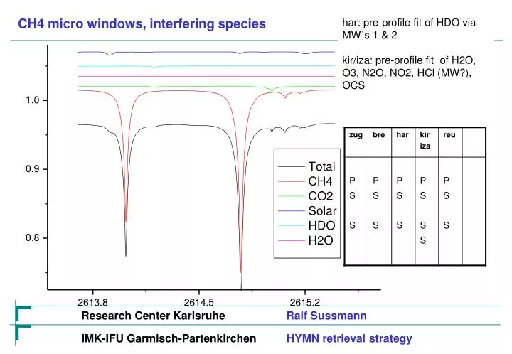
CH4 micro windows, interfering species. har: pre-profile fit of HDO via MW´s 1 & 2 kir/iza: pre-profile fit of H2O, O3, N2O, NO2, HCl (MW?), OCS. CH4 micro windows, interfering species. CH4 micro windows, interfering species. HDO. CH4 micro windows, interfering species. ?. ?. HDO. H2O.

E N D
CH4 micro windows, interfering species har: pre-profile fit of HDO via MW´s 1 & 2 kir/iza: pre-profile fit of H2O, O3, N2O, NO2, HCl (MW?), OCS
CH4 micro windows, interfering species ? ? HDO H2O
At ZUG we don´t find a significant impact of joint profile retrieval of H2O, HDO versus scaling (others?) H2O dofs=3, HDO dofs=1 H2O dofs=1, HDO dofs=1 AVi(i) = 0.501 AVi(i) = 0.521 H2O dofs=1, HDO dofs=3 AVi(i) = 0.504
At ZUG we don´t find a significant impact of ECMW versus Munich radio sonde (others?) Munich radio sonde ECMWF Sigma i 0.516868287 0.518528544 Sigma i/sqrt(ni) 0.24454497 0.244846405 day-to-day 0.786555915 0.766957709 Munich radio sonde ECMWF
At ZUG we find a very small reduction of the diurnal variation using Frankenberg versus HITRAN 04 line data stdv of diurnal variation AVi(i)
At ZUG we don´t se obvious impact on profiles using Frankenberg versus HITRAN 04 line data (others?) HITRAN 04 Frankenberg fit line data dofs = 2 dofs = 2 dofs = 3 dofs = 3
Bremen and Reunion (dofs 2, diagonal Sa) are significantly unter-estimating true variability
There can be a significant a priori impact on your columns precision AVi (i) note strong a priori impact for profile scaling (dofs = 1) ( )
Input (I): provide mean tropopause altitude for your site Therefore we construct a set of consistent a priori´s which we provide to each station: We use the CH4 profile from reftoon corrected for tropopause altitude (via the linear transformation described in Arndt Meier´s thesis) Provide us the mean tropopause altitude for your station(s)
It is easy to under- / overestimate XCH4 day-to-day variability because of special regularization settings (e.g., diagonal Sa with dofs 2: Bremen, Reunion) ISSJ 2003 Reunion 04/07 Zugspitze 2003 dofs=2 detected day-to-day variability AVi (i) dofs=2.5 (daily means) diurnal variation dofs=3 (Thikonov-L1-tuning)
Input (II): provide kmat.dat (Kx, Se) from 15 different retrievals Therefore we construct a set of consistent R matrices for each station: We provide you a ready to use R matrix based upon the Tikhonov L1 operator wich is set in a way to yield dofs = 2 (or 2.5, to be decided) provide kmat.dat (Kx, Se) from 15 different retrievals with the Toon a priori adapted to your site. The ensemble should cover the full span of SZA´s and columns for your site
Input(III): prepare for years 2003 and 2004 four indiv. columns data sets: FTIR, SCIA 200 km, SCIA 500 km, SCIA 1000 km calculate XCH4 for FTIR by dividing CH4 column by daily air column (sum up 3rd block in fasmas file)
Input (V): calculate i of day i, average over all days i, separate numbers for 2003 & 2004; (we offer to do that for you, if you like) in per cent AVi (i) & AVi (i/sqrt(ni)) i of day i (18 Sep) = 0.13 % ni = 9 columns, 10 min integration per column XCH4
Input (VI): calculate sigma of day-to-day-variability for 2003 & 2004 separately; (we offer to do that for you, if you like) Zugspitze FTIR daily means (daily means) 0.8 % If there is a significant annual cycle: normalize first by dividing by 3rd order polynomial fit!
Input(IV): provide statistical numbers for SCIA, 2003 & 2004 separately (we offer to do that for you, if you like) 2003 SCIA all sigmas in % *pixels per day **first divide data by 3rd order polynomial fit to correct for annual cycle
SCIA IMPA-DOAS v49 now reflects our a priori understanding of the impact of pixel selection radius on columns variability Case a): (planetary-)wave length > selection radius Case b): (planetary-)wave length < selection radius tropopause altitude altitude z surface level selection radius north south an average of (SCIA) pixels witin a certain selection radius tends to see the same (case a) or slightly smaller (case b) day-to-day columns variability compared to a point-type measurement (Zugspitze FTIR)