Download
1 / 15
150 likes | 271 Vues
Clear Sky Forward Model & Its Adjoint Model. MURI Review April 27, 2004 leslie moy, dave tobin, paul van delst, hal woolf. Accomplishments:. Reproduce and Upgrade existing GIFTS/IOMI Fast Model • Coefficients promulgated 2003.

E N D
Clear Sky Forward Model & Its Adjoint Model MURI Review April 27, 2004 leslie moy, dave tobin, paul van delst, hal woolf
Accomplishments: Reproduce and Upgrade existing GIFTS/IOMI Fast Model • Coefficients promulgated 2003. • Greatly improved the dependent set statistics (esp. water vapor). • SVD regression and optical depth weighting incorporated. • Written in flexible code with visualization capabilities. Under CVS control. Write the Corresponding Tangent Linear and Adjoint Code • Tested to machine precision accuracy. • User friendly “wrap-around” code complete.
Fixed Gas Amounts Spectral line parameters Lineshapes & Continua Reduce to sensor’s spectral resolution Fast Model Coefficients, ci Fast Model Regressions Profile Database Compute monochromatic layer-to-space transmittances Layering, l Convolved Layer-to-Space Transmittances, tz (l) Fast Model Predictors, Qi Effective Layer Optical Depths, keff Fast Model Production Flowchart: keff = -ln (teff ) = Si=1:N ci Qi
------- GIFTS NeDT@296K ------- OSS RMS upper limit* Dependent Set Statistics: RMS(LBL-FM) current model MURI version MURI model w/ OD weighted SVD AIRS model c/o L. Strow, UMBC OSS model c/o Xu Liu, AER, Inc. OPTRAN, AIRS 281 channel set c/o PVD
User Input: User Output: Profile of temperature, ozone, water vapor at 101 levels Profileperturbation of temperature, ozone, water vapor at 101 levels Use to adjust initial profile Forward Model: Adjoint Model: Layer.m - convert 101 level values to 100 layer values Predictor.m - convert layer values to predictor values Calc_Trans.m - using predictors and coefficients calculate level to space transmittance Trans_to_Rad.m - calculate radiance Layer_AD.m - layer to level sensitivities Predictor_AD.m - level to predictor sensitivities Calc_Trans_AD.m - predictor to transmittance sensitivities Trans_to_Rad_AD.m - transmittance to radiance sensitivities User Output: User Input: Compare to observations Radiance Spectrum Radiance Spectrum perturbation
Simple Example: One Line Forward Model • Forward (FWD) model. The FWD operator maps the input state vector, X, to the model prediction, Y, e.g. for predictor #11: • Tangent-linear (TL) model. Linearisation of the forward model about Xb, the TL operator maps changes in the input state vector, X, to changes in the model prediction, Y, Or, in matrix form:
Using the same procedure as in the Simple Model, build up the Tangent Linear Model. Forward Model: TL Model: Layer.m - input: 101 level values of T,w,oz output: 100 layer values Predictor.m - input: layer values output: predictor values Calc_Trans.m - input: predictors, and coefficients output: transmittances Trans_to_Rad.m - input: transmittances output: TOA radiance Layer_TL.m - input: d(level value) output: d(layer value) Predictor_TL.m - input d(layer value), output: d(predictor), Calc_Trans_TL.m - input: d(predictor) output: d(transmittance) Trans_to_Rad_TL.m - input: d(transmittance) output: d(radiance) Testing subroutines: A range of Perturbations are added to a baseline input value. Plus&Minus 25% The Forward output (less the baseline value) is compared to the TL output.
TL testing for Dry Predictor #6 (T2) vs Temp at layer 44.* TL results must be linear.* TL must equal (FWD-To) at dT=0. TL results = blue, FWD-T0 results = red Difference between TL and FWD Input Temperature at Layer 44 were varied 25%.
TL testing for Dry Predictor #6 vs Temp at all layers.Similar plots made for each subroutine’s variables. D(dry.pred#6) Layer no. D(temp), %
Adjoint (AD) model. The AD operator maps in the reverse direction where for a given perturbation in the model prediction, Y, the change in the state vector, X, can be determined. The AD operator is the transpose of the TL operator. Using the example for predictor #11 in matrix form, Expanding this into separate equations:
Adjoint code testing for Dry Predictor #6 vs Temperature layer.AD - TLt residual must be zero.Similar plots are produced for every subroutine’s variables. AD - TLt residual Output variable layer Input variable layer
Adjoint for US Standard Profile, d(radiance)/d(ozone) Pressure, -mbar Wavenumber, cm-1
Adjoint for US Standard Profile, d(radiance)/d(water vapor) Pressure, -mbar Wavenumber, cm-1
Future Goals: ‘Reproduce and Upgrade existing GIFTS Fast Model’ • Increase the number and quality of training profiles (48); extend satellite zenith angle range; further improve the dependent and independent set statistics. • Breakout other gases. • Steer research direction based on user feedback. Corresponding Tangent Linear and Adjoint Code • Improve code for speed and ease of use. Convert to a more efficient programming language. • Investigator testing of code.
Adjoint code can be used for sensitivity analysis.d(Dry Predictor #6) / d(layer Temperature). Sensitivity, d(P6)/d(T) Output variable layer Input variable layer