Download
1 / 38
420 likes | 697 Vues
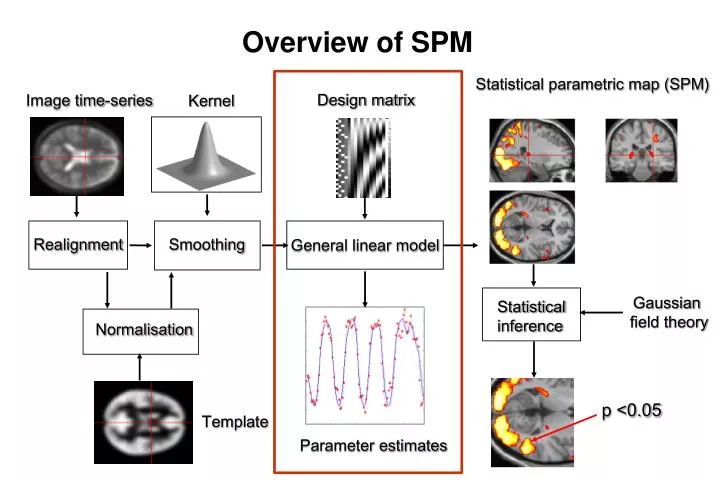
Overview of SPM. Statistical parametric map (SPM). Design matrix. Image time-series. Kernel. Realignment. Smoothing. General linear model. Gaussian field theory. Statistical inference. Normalisation. p <0.05. Template. Parameter estimates. The General Linear Model (GLM).

E N D
Overview of SPM Statistical parametric map (SPM) Design matrix Image time-series Kernel Realignment Smoothing General linear model Gaussian field theory Statistical inference Normalisation p <0.05 Template Parameter estimates
The General Linear Model (GLM) Frederike Petzschner Translational Neuromodeling Unit (TNU)Institute for Biomedical Engineering, University of Zurich & ETH Zurich With many thanks for slides & images to: FIL Methods group, Virginia Flanagin and KlaasEnno Stephan
Image a very simple experiment… • Onesession • 7 cyclesofrestandlistening • Blocks of 6 scanswith7 sec TR time
Image a very simple experiment… What we measure. single voxel time series Time What we know. time Question: Isthere a change in the BOLD responsebetweenlisteningandrest?
Image a very simple experiment… What we measure. single voxel time series Time What we know. time Question: Isthere a change in the BOLD responsebetweenlisteningandrest?
You need a model of your data… linear model effectsestimate statistic errorestimate Question: Isthere a change in the BOLD responsebetweenlisteningandrest?
Explain your data… as a combination of experimental manipulation,confounds and errors error = + + 1 2 Time e x1 x2 BOLD signal regressor Single voxel regression model:
Explain your data… as a combination of experimental manipulation,confounds and errors error = + + 1 2 Time e x1 x2 BOLD signal Single voxel regression model:
The black and white version in SPM 1 error 2 p = + Designmatrix + error 1 n n n e p 1 1 n: numberofscans p: numberofregressors
Model assumptions The design matrix embodies all available knowledge about experimentally controlled factors and potential confounds. Talk: Experimental Design Wed 9:45 – 10:45 Designmatrix You want to estimate your parameters such that you minimize: This can be done using an Ordinary least squaresestimation (OLS) assuming an i.i.d. error: error
error GLM assumes identical and independently distributed errors i.i.d. = errorcovarianceis a scalar multiple oftheidentitymatrix: Cov(e) = 2I non-identity non-independence t1 t2 t1 t2
How to fit the model and estimate the parameters? error „Option 1“: Per hand = + X y
How to fit the model and estimate the parameters? OLS (Ordinary Least Squares) error Data predicted by our model Error between predicted and actual data Goal is to determine the betas such that we minimize the quadratic error = + X y
OLS (Ordinary Least Squares) The goal is to minimize the quadratic error between data and model
OLS (Ordinary Least Squares) The goal is to minimize the quadratic error between data and model
OLS (Ordinary Least Squares) The goal is to minimize the quadratic error between data and model This is a scalar and the transpose of a scalar is a scalar
OLS (Ordinary Least Squares) The goal is to minimize the quadratic error between data and model This is a scalar and the transpose of a scalar is a scalar
OLS (Ordinary Least Squares) The goal is to minimize the quadratic error between data and model This is a scalar and the transpose of a scalar is a scalar You find the extremum of a function by taking its derivative and setting it to zero
OLS (Ordinary Least Squares) The goal is to minimize the quadratic error between data and model This is a scalar and the transpose of a scalar is a scalar You find the extremum of a function by taking its derivative and setting it to zero SOLUTION: OLS of the Parameters
A geometric perspective on the GLM OLS estimates y e x2 x1 Design space defined by X
Correlated and orthogonal regressors y Design space defined by X x2 x2* x1 Correlated regressors = explained variance is shared between regressors When x2 is orthogonalized with regard to x1, only the parameter estimate for x1 changes, not that for x2!
We are nearly there… linear model effectsestimate statistic errorestimate = +
What are the problems? Design Error • BOLD responses have a delayed and dispersed form. • The BOLD signal includes substantial amounts of low-frequency noise. • The data are serially correlated (temporally autocorrelated) this violates the assumptions of the noise model inthe GLM
Problem 1: Shape of BOLD response The response of a linear time-invariant (LTI) system is the convolution of the input with the system's response to an impulse (delta function).
Solution: Convolution model of the BOLD response expected BOLD response = input function impulse response function (HRF) HRF blue= data green= predicted response, taking convolved with HRF red= predicted response, NOT taking into account the HRF
Problem 2: Low frequency noise blue= data black = mean + low-frequency drift green= predicted response, taking into account low-frequency drift red= predicted response, NOT taking into account low-frequency drift
Problem 2: Low frequency noise Linear model blue= data black = mean + low-frequency drift green= predicted response, taking into account low-frequency drift red= predicted response, NOT taking into account low-frequency drift
Solution 2: High pass filtering discrete cosine transform (DCT) set
Problem 3: Serial correlations i.i.d non-independence non-identity t1 t2 t1 t2 n n n: numberofscans
Problem 3: Serial correlations with 1st order autoregressive process: AR(1) autocovariance function n n n: numberofscans
Problem 3: Serial correlations • Pre-whitening: 1. Use an enhanced noise model with multiple error covariance components, i.e. e ~ N(0,2V) instead of e ~ N(0,2I).2. Use estimated serial correlation to specify filter matrix W for whitening the data. This is i.i.d
How do we define W ? • Enhanced noise model • Remember linear transform for Gaussians • Choose W such that error covariance becomes spherical • Conclusion: W is a simple function of V so how do we estimate V ?
Find V: Multiple covariance components enhanced noise model error covariance components Q and hyperparameters V Q2 Q1 1 + 2 = Estimation of hyperparameters with EM (expectation maximisation) or ReML(restricted maximum likelihood).
We are there… linear model effectsestimate statistic errorestimate • GLM includes all known experimental effects and confounds • Convolution with a canonical HRF • High-pass filtering to account for low-frequency drifts • Estimation of multiple variance components (e.g. to account for serial correlations) = +
We are there… c = 1 0 0 0 0 0 0 0 0 0 0 linear model Null hypothesis: effectsestimate statistic errorestimate Talk: Statistical Inference and design efficiency. Next Talk = +
We are there… • Mass-univariate approach: GLM applied to > 100,000voxels • Threshold of p<0.05 more than 5000 voxels significant by chance! single voxel time series Time • Massive problem with multiple comparisons! • Solution: Gaussian random field theory
Outlook: further challenges • correction for multiple comparisons Talk: Multiple Comparisons Wed 8:30 – 9:30 • variability in the HRF across voxels Talk: Experimental Design Wed 9:45 – 10:45 • limitations of frequentiststatistics Talk: entire Friday • GLM ignores interactions among voxels Talk: Multivariate Analysis Thu 12:30 – 13:30
Thank you! Read me • Friston, Ashburner, Kiebel, Nichols, Penny (2007) Statistical Parametric Mapping: The Analysis of Functional Brain Images. Elsevier. • Christensen R (1996) Plane Answers to Complex Questions: The Theory of Linear Models. Springer. • Friston KJ et al. (1995) Statistical parametric maps in functional imaging: a general linear approach. Human Brain Mapping 2: 189-210.