Download
1 / 63
630 likes | 761 Vues
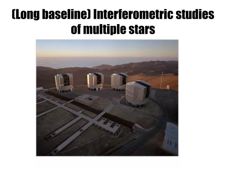
(Long baseline) Interferometric studies of multiple stars. Overview. Stellar Interferometry and the ESO paradigm Advances in modeling Application to SB2s Challenges and rewards of multiple stars Using interferometry Interferometry with VLTI. Overview. Stellar Interferometry

E N D
Overview • Stellar Interferometry and the ESO paradigm • Advances in modeling • Application to SB2s • Challenges and rewards of multiple stars • Using interferometry • Interferometry with VLTI
Overview • Stellar Interferometry • Interferometers of the world and the ESO paradigm • What is an interferometer • Responses to simple models (direct problem) • Aperture synthesis and imaging • Visibility functions in the aperture plane • Advances in modeling • Application to SB2s • Challenges and rewards of multiple stars • Using interferometry • Interferometry with the VLTI
Interferometers of the world VLTI Keck CHARA NPOI IOTA COAST SUSI GI2T PTI
What is an interferometer? http://sim.jpl.nasa.gov/interferometry/Demo
Definition of Complex Visibility V = (Pmax – Pmin ) / (Pmax + Pmin )
Stellar interferometer Van Cittert – Zernike Theorem The complex degree of coherence measured by an interferometer baseline is equal to a single spatial frequency of the Fourier transform of the object brightness distribution.
Responses to simple models • Point source (“unresolved”) º constant • Uniform disk • Elliptical disk • Limb darkened disk • Binary (and higher multiples) • Gaussian = Gaussian
Elliptical disk Transform (u,v) coord. Fourier transform strip brightness distribution van Belle et al. (2001)
Limb darkened disk Wittkowski et al. (2003)
Binary Mark III
Aperture Synthesis Earth’s rotation changes a baselines orientation and projected length relative to the source. Thus, with a multi- element interferometer, an aperture much larger than that of a single telescope can be synthesized.
Phase closure The atmosphere corrupts the visibility phase by adding random phase offsets above each aperture. The sum of the phase in a closed triangle of baselines is free of atmospheric effects and therefore equal to that of the object.
Aperture plane visibility functions • Equal magnitude binary • Resolved component in binary • Faint secondary vs resolved primary • Triple star
Visibility functions (1) Equal magnitude double star.
Visibility functions (2) Wide equal magnitude double star with resolved component.
Visibility functions (3) Wide double star with faint secondary and resolved primary.
Visibility functions (4) Triple system, unresolved components.
Overview • Stellar Interferometry and the ESO paradigm • Advances in modeling • Interferometric data • Combining spectroscopic and interferometric data • Application to SB2s • Challenges and rewards of multiple stars • Using interferometry • Interferometry with VLTI
Atlas (Pleiades) Hipparcos distance: 118.3 +/- 3.5 pc From orbital parallax: 132 +/- 4 pc (ELODIE,CORALIE,FEROS + KOREL) Zwahlen et al. 2004 (MARK III, NPOI)
b Centauri (B1III + B1III) M= 9.1 (14.4) Davis et al. 2005 (SUSI) Ausseloos et al. 2002
Aperture synthesis and orbital motion Mark III single night obervation Motion of P=4d secondary in one night.
Visibility fitting (Iota Peg: Boden et al. 1999)
ο Leonis combined fitting Elements Physical parameters
Fundamental stellar parameters (z Aurigae) Bennett et al. 1996
Overview • Stellar Interferometry • Advances in modeling • Application to SB2s • Precision of masses • Orbital parallaxes • Footprints in the HR diagram • Challenges and rewards of multiple stars • Using interferometry • Interferometry with the VLTI
Overview • Stellar Interferometry • Advances in modeling • Application to SB2s • Challenges and rewards of multiple stars • Field of view issues • Hierarchical model • Orbit orientations • Using interferometry • Interferometry with the VLTI
Interferometry of triple stars h Vir (Hummel et al. 2003)
Orbital motion in h Virginis Images from NPOI data (Hummel et al. 2003)
Orbits in h Virginis P = 4794 d P = 71 d
Hierarchical Model Format Stellar parameters Orbital elements
Reference orbits of Aa and Ab to B. M(Aa) / M(Ab) = 1.27 +/- 0.09 From spectroscopy: M(Aa) / M(Ab) = 1.33 +/- 0.02 Mass ratio from astrometry
Stellar masses for h Virginis Aa-Ab is double lined: Obtain all three masses with spectroscopy. Determine relative orbit orientations by identifying ascending node
Overview • Stellar Interferometry and the ESO paradigm • Advances in modeling • Double-lined spectroscopic binaries • Challenges and rewards of multiple stars • Using interferometry • Interferometers as telescopes • Interpretation of interferometric data (inverse problem) • Interferometry with VLTI
Interferometers as telescopes • Photometric field of view • Interferometric field of view • Broadband aperture synthesis • Sparse sampling does not allow model independent imaging • Sensitivity: it’s the correlated flux! Courtesy of Tyler Nordgren
Photometric field of view Mizar A (V=2.3) with B (V=4.0) at 14” (Mark III)
Interferometric field of view 12 Persei observed on Oct 9, 2001 with the CHARA Array, K’-band, 330m baseline, separation 40 marcsec Mark 3 (Oct 8, 1992)
Interferometric field of view b CrB (NPOI)
Broadband aperture synthesis h Peg (NPOI) h Peg
Overview • Stellar Interferometry and the ESO paradigm • Advanced modeling • Double-lined spectroscopic binaries • Challenges and rewards of multiple stars • Using interferometry • Interferometry with VLTI • Layout • Instrumentation
Existing VLTI instruments • VINCI: 2-channel (H & K) fiber 2-beam combiner • Commissioning only • MIDI: R=30-260 (8 – 13μ) 2-beam combiner • offered to astronomers first in P73 • AMBER: R= 35 – 14000, JHK, 3 telescope combiner • First offered for P76
MIDIoverview MIDI Overview MIDI [D/F/NL; PI: Heidelberg] Paranal:November 2002 First Fringes with UTs:December 2002 Mid IR instrument (10–20 mm) , 2-beam, Spectral Resolution: 30-260 Limiting Magnitude N ~ 4 (1.0Jy, UT with tip/tilt, no fringe-tracker) (0.8 AT) N ~ 9 (10mJ, with fringe-tracker) (5.8 AT) Visibility Accuracy 1%-5% Airy Disk 0.26” (UT), 1.14” (AT) Diffraction Limit [200m] 0.01”