Formulating Semantic Image Annotation as a Supervised Learning Problem Gustavo Carneiro and Nuno Vasconcelos CVPR ‘05

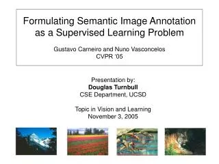
1. Formulating Semantic Image Annotation as a Supervised Learning ProblemGustavo Carneiro and Nuno VasconcelosCVPR ‘05 Presentation by: Douglas Turnbull CSE Department, UCSD Topic in Vision and Learning November 3, 2005

2. What is Image Annotation? Given an image, what are the words that describe the image?

3. What is Image Retrieval? Given a database of images and a query string (e.g. words), what are the images that are described by the words? Query String: “jet”

4. Problem: Image Annotation & Retrieval Based on the low cost of both digital camera and hard disk space, billions of consumer have the ability create and store digital images. There are already billions of digital images stored on personal computers and in commercial databases. How do store images in and retrieve images from a large database?

5. Problem: Image Annotation & Retrieval In general, people do not spent time labeling, organizing or annotating their personal image collections. Label: • Images are often stored with the name that is produced by the digital camera: • “DSC002861.jpg” • When they are labeled, they are given a vague names that rarely describe the content of the image: • ”GoodTimes.jpg”, “China05.txt” Organize: • No standard scheme exists for filing images • Individuals use ad hoc methods: “Chrismas2005Photos” and “Sailing_Photos” • It is hard to merge image collections since the taxonomies (e.g. directory hierarchies) differ from user to user.

6. Problem: Image Annotation & Retrieval In general, people do not spent time labeling, organizing or annotating their personal image collections. Annotate: • Explicit Annotation: Rarely do we explicitly annotate our images with captions. • An exception is when we are create web galleries • i.e. My wedding photos on www.KodakGallery.com • Implicit Annotation: Sometimes we do implicitly annotate images we imbed images into text (as is the case with webpages.) • Web-based search engines make use of the implicit annotation when they index images. • i.e. Google Image Search, Picsearch

7. Problem: Image Annotation & Retrieval If we can’t depend on human labeling, organization, or annotation, we will have to resort to “content-based image retrieval”: • We will extract features vectors from each image • Based on these feature vectors, we will use statistical models to characterize the relationship between a query and image features. How do we specify a meaningful query to be able to navigate this image feature space?

8. Problem: Image Annotation & Retrieval Content-Based Image Retrieval: How do we specify a query? Query-by-sketch: Sketch a picture, extract features from the pictures, we the features to find similar images in the database. This requires that • we have a good drawing interface handy • everybody is able to draw • the quick sketch is able to capture the salient nature of the desired query Not a very feasible approach.

9. Problem: Image Annotation & Retrieval Content-Based Image Retrieval: How do we specify a query? Query-by-text: Input words into a statistical model that models models the relationship between words and image features. This requires that: 1. A keyboard 2. A statistical model that can relate words to image features 3. Words can be used to capture the salient nature of the desired query. A number of research systems have been develop that find a relationship content-based image features and text for the purpose of image annotation and retrieval. - Mori, Takahashi, Oka (1999) - Daygulu, Barnard, de Freitas (2002) - Blei, Jordan (2003) - Feng, Manmantha, Lavrenko (2004)

10. Outline Notation and Problem Statement Three General Approaches to Image Annotation • Supervised One vs. All (OVA) Models • Unsupervised Models using Latent Variables • Supervised M-ary Model Estimating P(image features|words) Experimental Setup and Results Automatic Music Annotation

11. Outline Notation and Problem Statement Three General Approaches to Image Annotation • Supervised One vs. All (OVA) Models • Unsupervised Models using Latent Variables • Supervised M-ary Model Estimating P(image features|words) Experimental Setup and Results Automatic Music Annotation

12. Notation and Problem Statement

13. Notation and Problem Statement Image and Caption Image Regions xi = vector of image features x = {x1, x2, …} = vector of feature vectors wi = one word w = {w1, w2, …} = vector of words

14. Notation and Problem Statement

15. Notation and Problem Statement -

16. Notation and Problem Statement Weak Labeling: this image depict sky eventhough the caption does contain “sky” Image Regions Multiple Instance Learning: this regions has no visual aspect of “jet”

17. Outline Notation and Problem Statement Three General Approaches to Image Annotation • Supervised One vs. All (OVA) Models • Unsupervised Models using Latent Variables • Supervised M-ary Model Estimating P(image features|words) Experimental Setup and Results Automatic Music Annotation

18. Supervised OVA Models Early research posed the problem as a supervised learning problem: train a classifier for each semantic concept. Binary Classification/Detection Problems: • Holistic Concepts: landscape/cityscape, indoor/outdoor scenes • Object Detection: horses, buildings, trees, etc Much of the early work focused on feature design and used existing models developed by the machine learning community (SVM, KNN, etc) for classification.

19. Supervised OVA Models

20. Supervised OVA Models • Pro: • Easy to implement • Can design features and tune learning algorithm for each classification task • Notion of optimal performance on each task • Data sets represent basis of comparison – OCR data set • Con: • Doesn’t scale well with a large vocabulary • Requires train and use L classifier • Hard to compare posterior probabilities output by L classifier • No natural ranking of keywords. • Weak labeling is a problem: • Images not labeled with keyword are placed in D0

21. Unsupervised Models The goal is to estimate the joint distribution We introduce a latent (e.g. hidden) variable L that encode S hidden states of the world. i.e. “Sky” state, “Jet” state A state defines a joint distribution of image features and keywords. i.e. P(x=(blue, white, fuzzy), w=(“sky”, “cloud”,”blue”) | “Sky” State) will have high probability. We can sum over the S states variable to find the joint distribution Learning is based on the expectation maximization (EM): 1) E-step: update strength of association between image-caption with state 2) M-step: maximize likelihood of joint distribution for each state Annotation involves the most probable words under the joint distribution model

22. Unsupervised Models Multiple-Bernoulli Relevance Model (MBRM) – (Feng, Manmantha, Lavrenko CVPR ’04) • Simplest unsupervised model which achieves best results • Each of the D images in the training set is a “not-so-hidden” state • Assume conditional independence between image features and keywords given state MBRM eliminates the need for EM since we don’t need to find the strength of association between image-caption and state. Parameter estimation is straight forward PX|L is estimated using a Gaussian kernel PW|L reduces to counting The algorithm becomes essentially “smoothed k-nearest neighbor”.

23. Unsupervised Models Pros: • More scaleable than Supervised OVA • Size of vocabulary • Natural ranking of keywords • Weaker demands on quality of labeling • Robust to a weakly labeled dataset Cons: • No guarantees of optimality since keywords are not explicitly treated as classes • Annotation: What is a good annotation? • Retrieval: What are the best images given a query string?

24. Supervised M-ary Model Critical Idea: Why introduce latent variables when a keyword directly represents a semantic class. A random variable W which takes values in {1,…,L} such that W = i if x is label with keyword wi. The class conditional distributions PX|W(x|i) are estimated using the images that have keyword wi. To annotate a new image with features x, the Bayes decision rule is invoked: Unlike Supervised OVA which consist of solving L binary decision problems, we are solving one decision problem with L classes. The keyword compete to represent the image features.

25. Supervised M-ary Model Pros: • Natural Ranking of Keywords • Similar to unsupervised models • Posterior probabilities are relative to same classification problem. • Does not require training of non-class models • Non-class model are the Yi = 0 in Supervised OVA • Robust to weakly labeled data set since images that contain concept but are not labeled with the keyword do not adversely effect learning. • Non-class models are computational bottleneck • Learning a density estimates PX|W(x|i) is computationally equivalent to learning density estimates for each image in MBRM model. • Relies on Mixture Hierarchy method (Vasconcelos ’01) • When vocabulary size (L) is smaller than the training set size (D), annotation is computationally more efficient than the most efficient unsupervised algorithm.

26. Outline Notation and Problem Statement Three General Approaches to Image Annotation • Supervised One vs. All (OVA) Models • Unsupervised Models using Latent Variables • Supervised M-ary Model Estimating P(image features|words) Experimental Setup and Results Automatic Music Annotation

27. Density Estimation For Supervised M-ary learning, we need to find the class-conditional density estimates PX|W(x|wi) using a training data set Di. • All the images in Di have been labeled with wi Two Questions: • Given that a number of the image regions from images in Di will not exhibit visual properties that relate to wi, can we even estimate these densities? i.e An image labeled “jet” will have regions where only sky is present. 2) What is the “best” way to estimate these densities? • “best” – the estimate can be calculated using a computationally efficient algorithm • “best” – the estimate is accurate and general.

28. Density Estimation Multiple Instance Learning: a bag of instance receive a label for the entire bag if one or more instances deserves that label. This makes the data noisy, but with enough averaging we can get a good density estimate. For example: 1 Suppose all images has three regions. 2 Every image annotated with “jet” have one region with jet-like features (i.e. mu =20, sigma = 3). 3 The other two regions are uniformly distributed with mu ~ U(-100,1000) and sigma ~ U(0.1,10) 4 If we average 1000 images, the “jet” distribution emerges

29. Density Estimation For word wi, we have Di images each of which is represented by a vector of feature vectors. The authors discuss four methods of estimating PX|W(x|i). • Direct Estimation • Model Averaging • Histogram • Naïve Averaging • Mixture Hierarchies

30. Density Estimation 1) Direct Estimation • All feature vectors for all images represent a distribution • Need to does some heuristic smoothing – e.g. Use a Gaussian Kernel • Does not scale well with training set size or number of vector per image Smoothed kNN Feature 2 Feature 1

31. Density Estimation 2) Model Averaging Each imagel in Di represents a individual distribution We average the image distributions to find one class distribution The paper mentions two techniques • Histograms – partition space and count • Data sparsity problems for high dimensional feature vectors. • Naïve Averaging using Mixture Models • Slow annotation time since there will be KD Gaussian if each image mixture has K components Smoothed kNN Histogram Mixtures Feature 2 Feature 2 Feature 2 Feature 1 Feature 1 Feature 1

32. Density Estimation 3) Mixture Hierarchies – (Vasconcelos 2001) • Each imagel in Di represents a individual mixture of K Gaussian distributions • We combine “redundant” mixture components using EM • E-Step: Compute weight between each of the KD components and the T components • M-Step: Maximize parameters of T components using weights • The final distribution is one Mixture of T Gaussians for each keyword wi where T << KD. Di l1 l2 l3 lDi . . .

33. Outline Notation and Problem Statement Three General Approaches to Image Annotation • Supervised One vs. All (OVA) Models • Unsupervised Models using Latent Variables • Supervised M-ary Model Estimating P(image features|words) Experimental Setup and Results Automatic Music Annotation

34. Experimental Setup Corel Stock Photos Data Set 5,000 images – 4,500 for training, 500 for testing Caption of 1-5 words per image from a vocabulary of L=371 keywords Image Features • Convert from RGB to YBR color space • Computes 8 x 8 discrete cosine transform (DCT) • Results is a 3*64 =192 dimensional feature vector for each image region • 64 low frequency features are retain so that

35. Experimental Setup Two (simplified) tasks: Annotation: given a new image, what are the best five words that describe the image Retrieval: Given a one word query, what are the images that match the query. Evaluation Metrics: |wH| - number of images that have been annotated with w by humans |wA| - number of images that have been automatically annotated with w |wC| - number of images that have been automatically annotated with w AND where annotated with w by humans Recall = |wC|/|wH| Precision = |wC|/|wA| Mean Recall and Mean Precision are average over all the words found in the test set.

36. Other Annotation Systems 1. Co-occurrence (1999) – Mori, Takahashi, Oka Early work that clusters sub-images (block-based decomposition) and counts word frequencies for each cluster 2. Translation (2002) – Duygulu, Barnard, de Freitas, Forsyth • “Vocabulary of Blobs” • Automatic Segmentation -> Feature Vectors -> Clustering -> Blobs • An image is made of of Blobs, Words are associated with Blobs -> New Caption • “Blobs” are latent states Block-Based Decomposition Automatic Decomposition

37. Other Annotation Systems 3. CRM (2003)- Lavrenko, Manmatha, Jeon Continuous-space Relevance Model “smoothed KNN” algorithm image features are modeled using kernel-based densities automatic image segmentation color, shape, texture features word features are modeled using multinomial distribution “Training Images” are latent states. 4. CRM-rect(2004) – Feng Manmantha, Lavrenko Same as CRM but using block-based decomposition rather than segmentation 5. MBRM (2004)– Feng, Manmantha, Lavrenko Multiple-Bernoulli Relevance Mode Same as CRM-rect but uses multiple-Bernoulli distribution to model word features shifts emphasis to presence of word rather than prominence of word.

38. New Annotation Systems 6. CRM-rect-DCT (2005) – Carneiro, Vasconcelos CRM-rect with DCT features 7. Mix-hier(2005) -Carneiro, Vasconcelos Supervised M-ary Learning Density estimation using Mixture Hierarchies DCT features

39. Annotation Results Examples of Image Annotations:

40. Annotation Results Performance of Annotation system on Corel test set 500 images, 260 keywords, generate 5 keywords per image Recall = |wC|/|wH|, Precision = |wC|/|wA| Gain of 16% recall at same or better level of precision Gain of 12% in words with positive recall i.e. a word is found in both human and automatic annotation at least once.

41. Annotation Results Annotation computation time for Mix-Hier scales with training set size. MBRM is O(TR), where T is training set size Mix-Hier is O(CR), where C is the size of the vocabulary R is the number of image regions per image. Complexity is measured in seconds to annotated a new images.

42. Retrieval Results First five ranked images for “mountain”, “pool”, “blooms”, and “tiger”

43. Retrieval Results Mean Average Precision For each word wi, find all na,i images that have been automatically annotated with word wi. Out of the na,i images, let nc,i be the number of images that have been annotated with wi by humans. The precision of wi is nc,i / na,i. If we have L words in our vocabulary, mean average precision is Mix-Hier does 40% better on words with positive recall.

44. Outline Notation and Problem Statement Three General Approaches to Image Annotation • Supervised One vs. All (OVA) Models • Unsupervised Models using Latent Variables • Supervised M-ary Model Estimating P(image features|words) Experimental Setup and Results Automatic Music Annotation

45. Automatic Music Annotation Annotation: Given a song, what are the words that describe the music. • Automatic Music Reviews Retrieval: Given a text query, what are the songs that are best describe by the query. • Song Recommendation, playlist generation, music retrieval Features extraction involves applying filters to digital audio signals Fourier, Wavelet, Gammatone are common filterbank transforms Music may be “more difficult” to annotate since music is inherently subjective. -Music evokes different thoughts and feeling to different listeners -An individual experience with music changes all the time -All music is art unlike most digital images. -The Corel data set consists of concrete “object” and “landscape” scene -An similar dataset might focus on Modern Art (Pollack, Mondrian, Dali)

46. Automatic Music Annotation Computer Hearing (aka Machine Listening, Computer Audition): • Music is one subdomain of sound • Sound Effects, Human speech, Animal Vocalization, Environment Sounds all represent other subdomains of sound • Annotation is one problem • Query-by-humming, Audio Monitoring, Sound Segmentation, Speech-to-Text are examples of other Computer Hearing Problems

47. Automatic Music Annotation Computer Hearing and Computer Vision are closely related: • Large public and private database exist that are rapidly growing in size • Digital Medium • Sound is 2D – intensity (amplitude) & time or frequency & magnitude • Sound is often represented in 3D – magnitude, time and frequency • Image is 3D – 2 spatial dimensions, an intensity (color) • Video is 4D – 2 spatial dimensions, an intensity, time • Video is comprised of both images and sound • Feature extraction techniques are similar • Applying filters to digital medium

48. Work Cited: Carneiro, Vasconcelos. “Formulating Semantic Image Annotation as a Supervised Learning Problem” (CVPR ’05) Vasconcelos. “Image Indexing with Mixture Hierarchies” (CVPR ’01) Feng, Manmatha, Lavernko. “Multiple Bernoulli Relevance Models for Image and Video Annotation” (CVPR ’04) Blei, Jordan. “Modeling Annotated Data” (SIGIR ’03)