Download
1 / 54
540 likes | 623 Vues
Sampling Distributions. Central Limit Theorem. Objectives. Investigate the variability in sample statistics from sample to sample. Find measures of central tendency for distribution of sample statistics. Find measures of dispersion for distribution of sample statistics.

E N D
Sampling Distributions Central Limit Theorem
Objectives • Investigate the variability in sample statistics from sample to sample • Find measures of central tendency for distribution of sample statistics • Find measures of dispersion for distribution of sample statistics. • Find the pattern of variability for sample statistics
Overview • A new sample mean can be calculated each time a new sample is taken • In this way, the sample mean can be analyzed as a random variable • Being able to calculate (approximately) the distribution of the sample mean is a critical tool for inference
Learning Objectives • Understand the concept of a sampling distribution • Describe the distribution of the sample mean for samples obtained from normal populations • Describe the distribution of the sample mean for samples obtained from a population that is not normal
Statistical Inference • Often the population is too large to perform a census … so we take a sample • How do the results of the sample apply to the population? • What’s the relationship between the sample mean and the population mean? • What’s the relationship between the sample standard deviation and the population standard deviation? • This is statisticalinference
Estimation • We want to use the sample mean to estimate the population mean μ • If we want to estimate the heights of eight year old girls, we can proceed as follows • Randomly select 100 eight year old girls • Compute the sample mean of the 100 heights • Use that as our estimate • This is using the sample mean to estimate the population mean
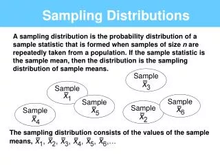
Sample Mean is a Variable • Usually, we just take one single sample to estimate population parameter. • However, if we take a series of different random samples from a target population • Sample 1 – we compute sample mean x1 • Sample 2 – we compute sample mean x2 • Sample 3 – we compute sample mean x3 • Etc. • Each time we sample, we may get a different result • The sample mean is a random variable!
Distribution of Sample Mean • Because the sample mean is a random variable • The sample mean has a probability distribution • We can obtain the center and spread of the probability distribution of the sample mean • This is called the distribution ofthesamplemean • Because the sample mean is a sample statistic, a distribution of a sample statistic is often called a sampling distribution. So, the distribution of the sample mean is also called sampling distribution of the mean.
Example 1 Consider a population of a uniformly distributed variable X with all of the values in the set {1, 2, 3, 4} occurring equally likely: • Calculate the mean and standard deviation of the population. • Make a list of all samples of size 2 that can be drawn from this set (Sample with replacement) • Construct the sampling distribution for the sample mean for samples of size 2 • Calculate the center and spread of the sampling distribution for the sample mean • Compare 1) and 4)
Example 1 (continued) • Mean of the population distribution of the variable X, denoted by mx or simply m: • Variance of the population distribution of the variable X, denoted by sx2 or simply s2 : • Standard deviation of the population distribution of the variable X, denoted by sx or simplys :
Example 1 (continued) This table lists all possible samples of size 2, the mean for each sample, and the probability of each sample occurring (all equally likely)
Sampling Distributionof the Sample Mean Histogram: Sampling Distributionof the Sample Mean Example 1 (continued) • Summarize the information in the previous table to obtain the sampling distribution of the sample mean : Notice that the sampling distribution of the sample mean is normal.
Example 1 (continued) • Mean of the sampling distribution of the sample mean , denoted by is: • Variance of the sampling distribution of the sample mean , denoted by is : • Standard deviation of the sampling distribution of the sample mean , denoted by is:
Example 1 (continued) From the above example, we conclude that • Sampling distribution of the sample mean tends to be bell-shaped. • The mean of the sampling distribution of the sample mean is the same as the underlying population mean. That is • The standard deviation of the sampling distribution of the sample mean is less than the standard deviation of the population standard deviation. In fact, Check:
Example 2 • We have the data 1, 7, 11, 12, 17, 17, 17, 21, 21, 21, 22, 22 and we want to take samples of size n = 3 • First, a histogram of the entire data set
Example 2 (continued) • A histogram of the entire data set • Definitely skewed left … not bell shaped
Example 2 (continued) • Taking some samples of size 3 • The first sample, 17, 21, 12, has a mean of 16.7 • The second sample, 17, 7, 17 has a mean of 13.7 • The third sample, 22, 11, 21 has a mean of 18
Example 2 (continued) • More sample means from more samples • We calculate the mean for each sample as shown below:
Example 2 (continued) • Finally, a histogram of 20 sample means
Example 2 (continued) • The original data set was highly left skewed, but the set of sample means is less skewed and closer to bell shaped
Example 2 (continued) • If taking a sample of size 5 repeatedly 20 times. • Here is a histogram of 20 sample means: Observe that the empirical distribution of sample means is more closer to bell shaped when the size of the sample increases.
Distribution of Sample Mean • In general, if the underlying population is closer to be bell shaped (normally distributed), then the sampling distribution (i.e. the distribution of sample mean) will tend to be more bell shaped as well. • In fact, the sampling distribution • Will be normally distributed • Will have a mean equal to the mean of the population • Will have a standard deviation less than the standard deviation of the population
Distribution of Sample Mean • Why does it have a smaller standard deviation? • The population standard deviation • Is a measure of the distance/deviation between an individual value and the population mean • Is a standard deviation of the sample mean for n = 1 • The standard deviation of the sample mean • Is a measure of the distance/deviation between the sample mean and the mean of the sampling distribution (which is the same as the population mean) • It makes sense that the estimate of the population mean using a sample mean is more accurate (closer to the population mean) if the sample contains more values (a larger n) from the population. Therefore, the larger the sample size, the less of the deviation of the sample mean from the true population mean. => standard deviation of sample mean is inversely related to the sample size n.
Sampling Distribution of Sample Mean • If a simple random sample of size n is drawn from a population, then the sampling distribution has • Mean x and • Standard deviation • In addition, if the population is normally distributed, then • The sampling distribution is normally distributed
Standard Error • The standard deviation of the sample mean is also called the standard error • The formula for is • This is an extremely important formula
Example • If the random variable X has a normal distribution with a mean of 20 and a standard deviation of 12 • If we choose samples of size n = 4, then the sample mean will have a normal distribution with a mean of 20 and a standard deviation of 6 (since ) • If we choose samples of size n = 9, then the sample mean will have a normal distribution with a mean of 20 and a standard deviation of 4 ( since ) Note: if the underlying population distribution is normal, the sampling Distribution of sample mean will be noraml regarless if the sample size is large or small.
Sampling Distribution of sample Mean • This is great if our random variable X has a normal distribution • However … what if underlying population distribution of the random variable X does not have a normal distribution • What can we say about the sampling distribution of the sample mean? • Wouldn’t it be very nice if the sampling distribution for sample mean also was normal? • This is almost true …
Central Limit Theorem • The CentralLimitTheorem states Regardless of the shape of the underlying population distribution, the sampling distribution of the sample mean becomes approximately normal as the sample size n increases. • Thus • If the random variable X is normally distributed, then the sampling distribution of the sample mean is normally distributed also regardless the size of the sample. • For all other random variables X, the sampling distributions are approximately normally distributed if the size of the sample is large enough.
Distribution of x:n = 2 Original Population 30 30 Distribution of x:n = 30 Distribution of x:n = 10 Graphical Illustration of the Central Limit Theorem
How large is the sample? • This approximation, of the sampling distribution being normal, is good for large sample sizes … large values of n • How large does n have to be? • A rule of thumb – if n is 30 or higher, this approximation is probably pretty good
Applications of the Central Limit Theorem • When the sampling distribution of the sample mean is (exactly) normally distributed, or approximately normally distributed (by the CLT), we can answer probability questions using the standard normal distribution.
Example 1 • We’ve been told that the average weight of giraffes is 2400 pounds with a standard deviation of 300 pounds • We randomly picked 50 giraffes and measured them and found that the sample mean was 2600 pounds • Is our data consistent with what we’ve been told? ( That is, does the sample mean of 2600 pounds observed support the claim that the average of population giraffes is 2400 pounds?)
Example 1 (continued) • Although we do not know the shape of the distribution of giraffe’s weight. Since the sample size is 50 which is large enough to justify the central limit theorem. The sampling distribution of the average weight of 50 giraffes is expected to be approximately normal with mean 2400 pounds (the same as the population) and a standard deviation of 300 / √ 50 = 42.4 pounds • Using our calculations for the general normal distribution, 2600 is 200 pounds over 2400, and 200 pounds is 200 / 42.4 = 4.7 . That is the Z-score for the average weight of 2600 is 4.7 which is a value near the end of the right tail of a standard normal distribution. • From our normal calculator, probability obtaining an average at least this large by chance is less than 0.00001. • Something is definitely strange … we’ll see what to do later in inferential statistics
1) 2) £ £ P ( 45 x 60 ) £ P ( x 47 . 5 ) Solutions: Since the original population is normal, the distribution of the sample mean is also (exactly) normal with • 1) m = m = 50 x • 2) s = s = = = n 15 9 15 3 5 x Example 2 Consider a normal population with m = 50 and s =15. Suppose a sample of size 9 is selected at random. Find: • use TI calculator to find the probability : • normalcdf(45,60,50,5) = 0.8186 • normalcdf(-E99,47.5,50,5) = 0.3085
x 45 50 60 - 2.00 1.00 0 - - æ ö 45 50 60 50 x - £ £ = £ £ z = ; z P ( 45 x 60 ) P ç ÷ è ø 5 5 s n = - £ £ P ( 1.00 z 2.00) = + = 0 . 3413 0 . 4772 0 . 8185 Example 2 (continued) Or, use Z-table to solve:
x 47.5 50 0 -0.50 - - æ ö x 50 47 . 5 50 x - £ = £ z = ; P ( x 47 . 5 ) P ç ÷ è ø 5 5 s n = £ - P ( z . 5 ) = - = 0 . 5000 0 . 1915 0 . 3085 Example 2 (continued)
m = m = s = s = » 109 n 20 50 2 . 83 x x Example 3 A recent report stated that the day-care cost per week in Boston is $109. Suppose this figure is taken as the mean cost per week and that the standard deviation is known to be $20. • Find the probability that a sample of 50 day-care centers would show a mean cost of $105 or less per week. • Suppose the actual sample mean cost for the sample of 50 day-care centers is $120. Is there any evidence to refute the claim of $109 presented in the report? Solutions: The shape of the original distribution is unknown, but the sample size, n = 50, is large. The CLT applies. The distribution of is approximately normal with
x - æ ö 105 109 x - z £ = £ z = ; P ( x 105 ) P ç ÷ è ø 2 . 83 s n = £ - P ( z 1 . 41 ) = - = 0 . 5000 0 . 4207 0 . 0793 Example 3 (continued) 1) Use Z-table: Or, Use TI calculator: normalcdf(-E99,105,109,2.83) = 0.0787
Consider how far out in the tail of the distribution of the sample mean is $120. æ - ö 120 109 ³ = z = ; z P ( x 120 ) P ç ³ ÷ è ø 2 . 83 = ³ P ( z 3 . 89 ) = 0.5000 - 0.4999 = 0.0001 x - s n Example 3 (continued) 2) • To investigate the claim, we need to examine how likely an observation is the sample mean of $120 Or using TI calculator: normalcdf(120,E99,120,2.83) = 5.08E-5 • Since the probability is so small, this suggests the observation of $120 is very rare (if the mean cost is really $109) • There is evidence (the sample) to suggest the claim of = $109 is likely wrong
Summary • The sample mean is a random variable with a distribution called the sampling distribution • If the sample size n is sufficiently large (30 or more is a good rule of thumb), then this distribution is approximately normal • The mean of the sampling distribution is equal to the mean of the underlying population • The standard error/deviation of the sampling distribution is equal to
Learning Objective • Describe the sampling distribution of a sample proportion • Calculate probabilities of a sample proportion
Sample Proportion • In an election, polling companies wish to estimate the percent of people who will vote for each candidate • This clearly is a situation for sampling as it is impractical to contact every single voter • The desired results are proportions, for example that 59% of the voters (a proportion of 0.59) said that they will vote for candidate A
Sampling Distribution of Sample Proportion • We have the same questions for the sample proportion as we had for the sample mean • What is the mean for the sampling distribution of the sample proportion? • What is the standard deviation for the sampling distribution of the sample proportion? • What is the distribution of the sample proportion? • Can we apply the Central Limit Theorem to approximate these with normal distributions? • The answer is yes …
Sample Proportions • A random sample is take • Of size n • Each individual either has or does not have a certain characteristic (dichotomous outcomes) • In total, there are x individuals that have this characteristic • Then the sampleproportion (p hat) (the proportion of individuals with this characteristic is given by
Example • If a polling company polled 800 people to see if they supported a certain issue and 475 did, then we have a sample proportion problem with • n = 800 • x = 475 • and a sample proportion of
Sampling Distribution of Sample proportion • If the population proportion is p, then the distribution of the sample proportion for a sample of size n • Is approximately normal if np(1-p) ≥ 10 • Has a mean of • Has a standard deviation of
Example • Assume that 80% of the people taking aerobics classes are female and a simple random sample of n = 100 students is taken • What is the probability that at most 75% of the sample students are female? • If the sample had exactly 90 female students, would that be unusual?
Example (continued) • The sample proportion of aerobics students who are female • Has an approximately normal distribution • Has a mean of 0.80 and a standard deviation of 0.04 • What is the probability that is 0.75 or less? • 0.75 is 0.05 less than the mean of 0.80 • 0.05 is 1.25 standard deviations less than the mean (i.e. the z-score is –1.25) • The normal probability P(z≤ –1.25) = .1056 • Thus P( ≤ 0.75) = .1056 Note: To obtain P( ≤ 0.75) = .1056, apply TI graphing calculator with normalcdf(-E99,-1.25,0,1) or normalcdf(-E99,0.75, 0.80,0.04) [or normalcdf(0,0.75,0.80,0.04),since probability can’t be less than zero.]