Quantity Theory of Money

1. Quantity Theory of Money

2. Why should the Quantity Theory of Money (QTM) be Introduced? • The QTM can be viewed as a special case of the economic theory behind the LM curve. • The equation behind the LM curve is that the real supply for money (M/P)s is equal to the real demand for money, and the demand of money depends on the transaction demand (i.e., it depends positively on output Y) and the speculative demand (i.e., it depends negatively on interest rate r)

3. Why should the Quantity Theory of Money (QTM) be Introduced? • A simple version of the QTM ignores the effects of interest rate and postulates that M/P = kY, where K is a positive constant. • The advantage of the QTM is that it explicitly brings in the relationship between the price level and the money supply and output. • This is important because as remarked by Milton Friedman, “Inflation is always and everywhere a monetary phenomenon.” Without the QTM, it is hard to discuss inflation.

4. Empirical Relevance of the QTM • How well does the QTM fit the empirical data, given that we ignore the effects of interest rate? Some variants of the QTM have been applied to many economies, including Hong Kong and China. It is known that the QTM works very well. • To empirically test the model, usually we need to modify the QTM a bit.

5. Empirical Relevance of the QTM • M/P = kY can be expressed in the form of m – p = y, where m is the % change in M, p is the % change in P, and y is the % change in Y. (Note that the growth rate of k must be zero because it is a constant.) Alternatively, p = m – y, i.e., inflation is positively related to growth rate in money supply and negatively related to output growth.

6. Empirical Relevance of the QTM • More advanced theories tell us that the real demand for money is better described by M/Pe, where Pe is expected inflation rate. This is because we don’t know what inflation is going to be, and so we can only form expectation of it. In practice, expected inflation rate depends on past values of actual inflation. Due to this complication, more sophisticated versions of the QTM assume that inflation depends on current and past values of the growth rates of M and Y. • This version of the QTM can explain more than 99% of the changes in prices in Hong Kong.

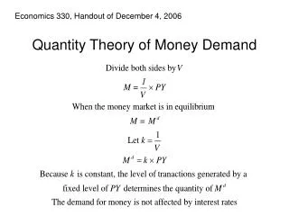
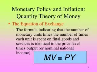
7. Earlier Versions of the QTM • Historically, the QTM has another form: MV = PY, where V is the velocity of money. It is supposed to measure how often the money stock turns over in each period. Alternatively, we can write V = nominal GDP/nominal money supply, i.e., V = PY/M. MV = PY should be treated as an identity, rather than an equation, because by the definition of V, it must always true. When there are changes in M, P, or Y, then V may have to adjust.

8. Earlier Versions of the QTM • Empirically, the V in the identity above need not be a constant. • If we impose the assumption that V is a constant, then we have the QTM, which can be tested empirically. The new version of the QTM is M/P = kY, where k = 1/V.