Download
1 / 44
450 likes | 575 Vues
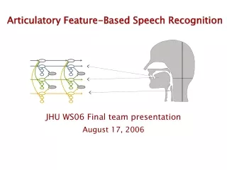
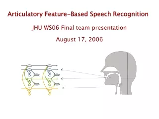
word. word. ind 1. ind 1. U 1. U 1. sync 1,2. sync 1,2. S 1. S 1. ind 2. ind 2. U 2. U 2. sync 2,3. sync 2,3. S 2. S 2. ind 3. ind 3. U 3. U 3. S 3. S 3. Articulatory Feature-Based Speech Recognition. JHU WS06 Final team presentation August 17, 2006. Project Participants.

E N D
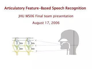
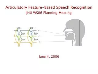
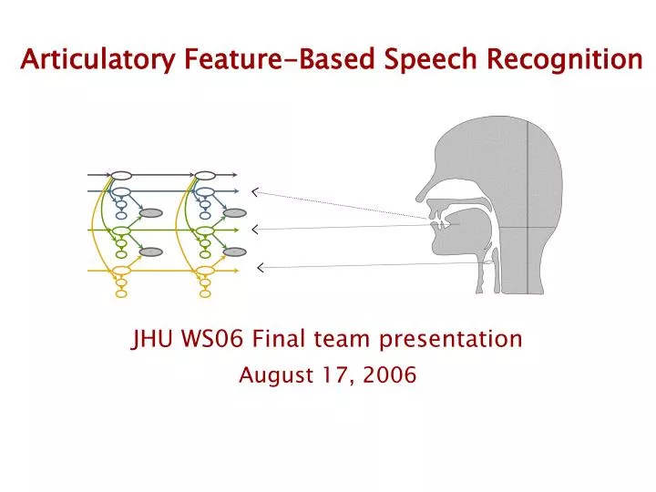
word word ind1 ind1 U1 U1 sync1,2 sync1,2 S1 S1 ind2 ind2 U2 U2 sync2,3 sync2,3 S2 S2 ind3 ind3 U3 U3 S3 S3 Articulatory Feature-Based Speech Recognition JHU WS06 Final team presentationAugust 17, 2006
Project Participants Team members: Karen Livescu (MIT) Arthur Kantor (UIUC) Özgür Çetin (ICSI) Partha Lal (Edinburgh) Mark Hasegawa-Johnson (UIUC) Lisa Yung (JHU) Simon King (Edinburgh) Ari Bezman (Dartmouth) Nash Borges (DoD, JHU) Stephen Dawson-Haggerty (Harvard) Chris Bartels (UW) Bronwyn Woods (Swarthmore) Advisors/satellite members: Jeff Bilmes (UW), Nancy Chen (MIT), Xuemin Chi (MIT), Trevor Darrell (MIT), Edward Flemming (MIT), Eric Fosler-Lussier (OSU), Joe Frankel (Edinburgh/ICSI), Jim Glass (MIT), Katrin Kirchhoff (UW), Lisa Lavoie (Elizacorp, Emerson), Mathew Magimai (ICSI), Daryush Mehta (MIT), Kate Saenko (MIT), Janet Slifka (MIT), Stefanie Shattuck-Hufnagel (MIT), Amar Subramanya (UW)
Outline • Preliminaries: Dynamic Bayesian networks, feature sets, data • Tandem AF-based observation models • Multistream AF-based pronunciation models
Why is this interesting? • Articulatory Featurres • Improved modeling of co-articulation • Potential savings in training data • Compatibility with more recent theories of phonology (autosegmental phonology, articulatory phonology) • Application to audio-visual and multilingual ASR • Improved ASR performance with feature-based observation models in some conditions [e.g. Kirchhoff ‘02, Soltau et al. ‘02] • Improved lexical access in experiments with oracle feature transcriptions [Livescu & Glass ’04, Livescu ‘05] • Tandem Models • Allow discriminative Training • Takes advantage of long-duration time windows (multiple frames) • Typically yields a large improvement in ASR accuracy
Yes No factored obs model? state asynchrony cross-word soft asynchrony soft asynchrony within word free within unit coupled state transitions Yes No [Livescu ‘04] [Deng ’97, Richardson ’00] fact. obs? fact. obs? fact. obs? fact. obs? obs model GM SVM NN N N N N Y Y Y Y [Metze ’02] [Kirchhoff ’02] [Juneja ’04] CD CD CD CD CD CD CD CD N N N Y N Y Y Y N Y N [Livescu ’05] N FHMMs ??? ??? Y N Y Y [WS04] [Kirchhoff ’96, Wester et al. ‘04] CHMMs ??? ??? ??? ??? ??? ??? ??? A (partial) taxonomy of design issues factored state (multistream structure)? ... plus, a variety of feature sets!
P(w) language model w = “makes sense...” pronunciation model P(q|w) q = [ m m m ey1 ey1 ey2 k1 k1 k1 k2 k2 s ... ] observation model P(o|q) o = Definitions: Pronunciation and observation modeling
A B C D Bayesian networks (BNs) • Directed acyclic graph (DAG) with one-to-one correspondence between nodes and variables X1, X2, ... , XN • Node Xi with parents pa(Xi) has a “local” probability function pXi|pa(Xi) • Joint probability = product of local probabilities: p(xi,...,xN) = p(xi|pa(xi)) p(b|a) p(a,b,c,d) = p(a)p(b|a)p(c|b)p(d|b,c) p(c|b) p(a) p(d|b,c)
frame i-1 frame i frame i+1 C C C A A B B A B D D D Dynamic Bayesian networks (DBNs) • BNs consisting of a structure that repeats an indefinite (i.e. dynamic) number of times • Useful for modeling time series (e.g. speech!)
FSN DBN frame i-1 frame i frame i+1 .7 .8 1 Qi-1 Qi+1 Qi .3 .2 . . . . . . P(qi|qi-1) P(obsi | qi) 1 2 3 obsi-1 obsi+1 obsi qi 1 2 3 qi-1 q=1 1 .7 .3 0 obs q=2 2 0 .8 .2 obs obs q=3 3 0 0 1 = variable = state = dependency = allowed transition Notation: Representations of HMMs as DBNs
word {“one”, “two” ,...} 1 wordTransition {0,1} 0 subWordState {0,1,2,...} stateTransition {0,1} phoneState {w1, w2, w3, s1,s2,s3,...} observation vector (MFCCs,PLPs) A phone HMM-based recognizer frame 0 frame i last frame variable name values • Standard phone HMM-based recognizer with bigram language model
Data • All experiments perfromed on 10 and 500 word training sets from the Svitchboard corpus • Svitchboard is small vocabulary subsets of switchboard
Articulatory feature sets • We use separate feature sets for pronunciation and observation modeling • Why? • For observation modeling, want features that are acoustically distinguishable • For pronunciation modeling, want features that can be modeled as independent streams
TB-LOC TT-LOC TB-OP TT-OP LIP-LOC VELUM LIP-OP GLOTTIS Feature set for pronunciation modeling • Based on articulatory phonology [Browman & Goldstein ‘90] adapted for pronunciation modeling [Livescu ’05] • Under some simplifying assumptions, can combine into 3 streams
Introduction • Tandem is a method to use the predictions of a MLP as observation vectors in generative models, e..g. HMMs • Extensively used in the ICSI/SRI systems: 10-20 % improvement for English, Arabic, and Mandarin • We explore tandem based on articulatory MLPs • Similar to the approach in Kirchhoff ’99 • Questions • Are articulatory tandems better than the phonetic ones? • Are factored observation models for tandem and acoustic (e.g. PLP) observations better than the observation concatenation approaches?
Tandem models: standard method • Standard phone-based tandem • Train an MLP to classify phonemes, frame by frame • Use the MLP output in tandem with PLPs as the observation vector Tandem models: our method • Feature-based tandem • Use ANNs to classify articulatory features instead of phones • 8 MLPs, classifying pl1, dg1, etc frame-by-frame One of the motivations for using features is that it should be easier to build a multi-lingual / cross-language system this way
training the MLPs • We use MLPs to classify speech into AFs, frame-by-frame • Must obtain targets for training • These are derived from phone labels • obtained by forced alignment using the SRI recogniser • this is less than ideal, but embedded training might help (results later) • MLPs were trained by Joe Frankel (Edinburgh/ICSI) & Mathew Magimai (ICSI) • Standard feedforward MLPs • Trained using Quicknet • Input to nets is a 9-frame window of PLPs (with VTLN and per-speaker mean and variance normalisation)
MLP details MLP architecture is: input units x hidden units x output units
MLP overall accuracies • Frame-level accuracies • MLPs trained on Fisher • Accuracy computed with respect to SVB test set • Silence frames excluded from this calculation • More detailed analysis coming up later…
MLP OUTPUTS LOGARITHM PRINCIPAL COMPONENT ANALYSIS SPEAKER MEAN/VAR NORMALIZATION TANDEM FEATURE Tandem Processing Steps • MLP posteriors are processed to make them Gaussian like • There are 8 articulatory MLPs; their outputs are joined together at the input (64 dims) • PCA reduces dimensionality to 26 (95% of the total variance) • Use this 26-dimensional vector as acoustic observations in an HMM or some other model • The tandem features are usually used in combination w/ a standard feature, e.g. PLP
State Concatenated Observations Factored Observations State Tandem PLP PLP p(X, Y|Q) = p(X|Q) p(Y|Q) Tandem Tandem Observation Models • Feature concatenation: Simply append tandems to PLPs • All of the standard modeling methods applicable to this meta observation vector (e.g., MLLR, MMIE, and HLDA) • Factored models: Tandem and PLP distributions are factored at the HMM state output distributions - Potentially more efficient use of free parameters, especially if streams are conditionally independent • Can use e.g., separate triphone clusters for each observation
Articulatory vs. Phone Tandems • Monophones on 500 vocabulary task w/o alignments; feature concatenated PLP/tandem models • All tandem systems are significantly better than PLP alone • Articulatory tandems are as good as phone tandems • Articulatory tandems from Fisher (1776 hrs) trained MLPs outperform those from SVB (3 hrs) trained MLPs
Concatenation vs. Factoring • Monophone models w/o alignments • All tandem results are significant over PLP baseline • Consistent improvements from factoring; statistically significant on the 500 task
Triphone Experiments • 500 vocabulary task w/o alignments • PLP x Tandem factoring uses separate decision trees for PLP and Tandem, as well as factored pdf’s • A significant improvement from factoring over the feature concatenation approach • All pairs of results are statistically significant
phoneState KLT’ed log MLP outputs, separate from PLP outputs PLPs Observation factoring and weight tuning Factored tandem Results Dimensions of streams Fully factored tandem phoneState PLPs dg1 pl1 rd . . . log outputs of separate MLPs Dims after KLT account for 95% of variance
PLPs KLT’ed log MLP outputs, separate from PLP outputs PLPs dg1 pl1 rd . . . Weight tuning Factored Fully factored MLP weight= 1 Language model tuned for PLP weight=1 Weight tuning in progress
Weight tuning with amoeba algorithm (on-going) • Search over the (9-dimentional) space of weights with the amoeba algorithm • Does not require estimation of derivative
Tandem Summary • Tandem features w/ PLPs outperform PLPs alone for both monophones and triphones • 8-13 % relative improvements (statistically significant) • Articulatory tandems are as good as phone tandems - Further comparisons w/ phone MLPs trained on Fisher • Factored models look promising (significant results on the 500 vocabulary task) - Further experiments w/ tying, initialization - Judiciously selected dependencies between the factored vectors, instead of complete independence
Multi-stream AF-based pronunciation models q (phonetic state) • Phone-based o (observation vector) • AF-based qi (state of AF i) o (obs vector)
word don’t probably baseform p r aa b ax b l iy d ow n t (2) p r aa b iy (1) p r ay (1) p r aw l uh (1) p r ah b iy (1) p r aa l iy (1) p r aa b uw (1) p ow ih (1) p aa iy (1) p aa b uh b l iy (1) p aa ah iy (37) d ow n (16) d ow (6) ow n (4) d ow n t (3) d ow t (3) d ah n (3) ow (3) n ax (2) d ax n (2) ax (1) n uw ... surface (actual) Motivation: Pronunciation variation everybody sense s eh n s eh v r iy b ah d iy [From data of Greenberg et al. ‘96] (1) s eh n t s (1) s ih t s (1) eh v r ax b ax d iy (1) eh v er b ah d iy (1) eh ux b ax iy (1) eh r uw ay (1) eh b ah iy
Pronunciation variation and ASR performance • Automatic speech recognition (ASR) is strongly affected by pronunciation variation • Words produced non-canonically are more likely to be mis-recognized [Fosler-Lussier ‘99] • Conversational speech is recognized at twice the error rate of read speech [Weintraub et al. ‘96]
[t] insertion rule dictionary Phone-based pronunciation modeling • Address pronunciation variation issue by substituting, inserting, or deleting segments: • Suffer from low coverage of conversational pronunciations and sparse data • Partial changes are not well described [Saraclar et al. ‘03] increased inter-word confusability sense [ s eh n t s ] / s eh n s /
feature values GLO open critical open VEL closed open closed dictionary TB mid / uvular mid / palatal mid / uvular TT critical / alveolar mid / alveolar closed / alveolar critical / alveolar phone s eh n s feature values surface variant #1 GLO open critical open VEL closed open closed TB mid / uvular mid / palatal mid / uvular TT critical / alveolar mid / alveolar closed / alveolar critical / alveolar phone s eh n t s feature values surface variant #2 GLO open critical open VEL closed open closed TB mid / uvular mid-nar / palatal mid / uvular TT critical / alveolar mid-nar / alveolar closed / alveolar critical / alveolar phone s ih t s n Revisiting examples (example of feature asynchrony) (example of feature asynchrony + substitution)
Reminder: phone-based model frame 0 frame i last frame variable name values word {“one”, “two” ,...} 1 wordTransition {0,1} 0 subWordState {0,1,2,...} stateTransition {0,1} phoneState {w1, w2, w3, s1,s2,s3,...} observation (Note: missing pronunciation variants)
wordTransition word wordTransitionL subWordStateL async stateTransitionL phoneStateL wordTransitionT L subWordStateT stateTransitionT phoneStateT T Recognition with a multistream pronunciation model • Degree of asynchrony ≡ |subWordStateL - subWordStateG| • Forces synchronization at word boundaries • Allows only asnchrony, no substitutions • Differences from implemented model: • Additional feature stream (G) • Pronunciation variants • Word transition bookkeeping
A first attempt: 1-state monofeat • Analogous to 1-state monophone with minimum duration of 3 frames • All three states of each phone map to the same feature values • One state of asynchrony allowed between L and T, and between G and {L,T}
Results: 1-state monofeat • Much higher WER than monophone—possible remedies • Improved modeling with the same structure • Alternative structures • Cross-word asynchrony • Context-dependent asynchrony • Substitutions
3-State Monofeat • Monofeat usually maps all states of a phone to the same feature value
3-State Monofeat • 3 State Monofeat makes a unique feature value for each phone state
3-State Monofeat • Why? • Forces a sequence of states • Models context
AF pronunciation modeling Summary • Conceptually appealing model for pronunciation variation • Modeling AF asynchrony does not yield an accuracy improvement yet • Many other things can be tried (different AF parameter initialization, different AF feature sets, parameter tying)