Download
1 / 43
460 likes | 720 Vues
Space fractional Schrödinger equation for a quadrupolar triple Dirac - potential. Jeffrey D. Tare* and Jose Perico H. Esguerra National Institute of Physics, University of the Philippines, Diliman, Quezon City 1101 *Presenter. Presented at the 7th Jagna International Workshop

E N D
Space fractional Schrödinger equation for a quadrupolar triple Dirac- potential Jeffrey D. Tare* and Jose Perico H. Esguerra National Institute of Physics, University of the Philippines, Diliman, Quezon City 1101 *Presenter Presented at the 7th Jagna International Workshop Research Center for Theoretical Physics, Jagna, Bohol 6–9 January 2014
Objective Obtain the solutions to the time-independent space fractional Schrödinger equation for a quadrupolar triple Dirac- potential for all energies
Contents I. Time-independent space fractional Schrödinger equation A. Position representation B. Momentum representation II. Quadrupolar triple Dirac- potential III. Methodology IV. Solutions to the time-independent space fractional Schrödinger equation A. (bound state) B. (scattering state) V. Evaluation of some integrals in terms of Fox’s H-function VI. Summary
I. Time-independent space fractional Schrödinger equation A. Position representation (1) Riesz fractional derivative (2) Fourier-transform pair (3) When , , with m being the mass of the particle.
I. Time-independent space fractional Schrödinger equation B. Momentum representation (4) Fourier convolution integral (5) (6)
II. Quadrupolar triple Dirac- potential In the framework of standard quantum mechanics the quadrupolar triple Dirac-delta (QTD-delta) potential has been considered by Patil1 and has the form (7) Figure 1. QTD-delta potential 1S. H. Patil, Eur. J. Phys. 30, 629 (2009)
III. Methodology TISFSE with QTD-delta potential Fourier transform to obtain the corresponding momentum representation Consider the cases E < 0 for bound state and E ≥ 0 for scattering state For E < 0 obtain energy equations for V0 > 0 and V0 < 0 and solve graphically to determine the number of bound states For E ≥ 0 obtain an expression for the wave function Inverse Fourier transform the wave functions to obtain the corresponding position representation Obtain the wave function and normalize it Express the wave functions in terms of Fox’s H-function
IV. Solutions to the time-independent space fractional Schrödinger equation After Fourier transforming the TISFE with a QTD-delta potential the following expression for the wave function in the momentum representation is obtained: (8) where (9)
IV. Solutions to the time-independent space fractional Schrödinger equation For this case we define (10) Then (11) A. (bound state)
IV. Solutions to the time-independent space fractional Schrödinger equation A. (bound state) (12) with (13) (14)
IV. Solutions to the time-independent space fractional Schrödinger equation A. (bound state) To obtain nontrivial solutions we impose the condition (15) where (16)
IV. Solutions to the time-independent space fractional Schrödinger equation A. (bound state) Energy equation (17) where (18) (19) (20)
IV. Solutions to the time-independent space fractional Schrödinger equation A. (bound state) Figure 2. Plots of the functions and for some values of α and R = 2. Red dots mark the intersection points.
IV. Solutions to the time-independent space fractional Schrödinger equation A. (bound state) The wave function can be obtained by inverse Fourier transforming (21) that is, (22) with (23)
IV. Solutions to the time-independent space fractional Schrödinger equation A. (bound state) • To normalize the technique of de Oliveira et al.2 is adapted. Parseval’s theorem (24) 2E. C. de Oliveira, F. S. Costa, and J. Vaz, Jr., J. Math. Phys. 51, 062102 (2010)
IV. Solutions to the time-independent space fractional Schrödinger equation A. (bound state) For the wave function be normalized to unity, (25) with (26) (27)
IV. Solutions to the time-independent space fractional Schrödinger equation A. (bound state) Normalized wave function (28) where (29) (30)
IV. Solutions to the time-independent space fractional Schrödinger equation A. (bound state) Figure 3. Plots of the wave function as a function of for some values of α and W = Z = 2.
IV. Solutions to the time-independent space fractional Schrödinger equation A. (bound state) Consider the case when the strength of the QTD-delta potential . Let . Then the QTD-delta potential becomes (31) Figure 4. QTD-delta potential when V0 < 0
IV. Solutions to the time-independent space fractional Schrödinger equation A. (bound state) Equations for Cn (n = 0,1,2) (32) (33)
IV. Solutions to the time-independent space fractional Schrödinger equation A. (bound state) Energy equations (34) (35) where
IV. Solutions to the time-independent space fractional Schrödinger equation A. (bound state) Figure 4. Plots of the energy equation (34) for Q = 2 and some values of α. Red dots mark the intersection points.
IV. Solutions to the time-independent space fractional Schrödinger equation A. (bound state) Figure 5. Plots of the energy equation (35) for Q = 2 and some values of α. Red dots mark the intersection points.
IV. Solutions to the time-independent space fractional Schrödinger equation A. (bound state) Normalized wave function (36) where (37) (38)
IV. Solutions to the time-independent space fractional Schrödinger equation A. (bound state) Figure 6. Plots of the wave function as a function of for W = Z = 2 and some values of α.
IV. Solutions to the time-independent space fractional Schrödinger equation B. (scattering state) For this case define (39) and use the property of the delta-function to write (40)
IV. Solutions to the time-independent space fractional Schrödinger equation B. (scattering state) Equations for (41) where 42) (43)
IV. Solutions to the time-independent space fractional Schrödinger equation B. (scattering state) Equations for (44) (45) (46)
IV. Solutions to the time-independent space fractional Schrödinger equation B. (scattering state) Notation
IV. Solutions to the time-independent space fractional Schrödinger equation B. (scattering state) The wave function after inverse Fourier transforming now reads (47) where
IV. Solutions to the time-independent space fractional Schrödinger equation B. (scattering state) In terms of Fox’s H-function (48) with (49)
V. Evaluation of some integrals in terms of Fox’s H-function In terms of Fox’s H-function evaluate integral of the form (50) Mellin-transform pair (51) (52)
V. Evaluation of some integrals in terms of Fox’s H-function Mellin transform of (53) Definitions/properties (54) (55) (56)
V. Evaluation of some integrals in terms of Fox’s H-function Mellin transform of (57) Useful formulas (58) (59)
V. Evaluation of some integrals in terms of Fox’s H-function Mellin transform of (60)
V. Evaluation of some integrals in terms of Fox’s H-function Fox’s H-function3 Definition (61) (62) 3A. M. Mathai, R. K. Saxena, and H. J. Haubold, The H-Function: Theory and Applications (Springer, New York, 2009)
V. Evaluation of some integrals in terms of Fox’s H-function Fox’s H-function Important property (change of independent variable) (63)
V. Evaluation of some integrals in terms of Fox’s H-function Recall the Mellin transform of T(y) (64) Inverse transform (65)
V. Evaluation of some integrals in terms of Fox’s H-function Identification of indices and parameters
V. Evaluation of some integrals in terms of Fox’s H-function Comparison with the definition of Fox’s H-function (66) (67)
VI. Summary • The time-independent space fractional Schrödinger equation for a QTD-delta potential is solved for all energies. • For the case E < 0 equations satisfied by the bound-state energy are derived. • Graphical solutions show that, for V0 > 0, there is only one bound-state energy for each fractional order α considered; and, for V0 < 0, there are two bound-state energies for each fractional order α considered. All the eigenenergies shift to higher values as α decreases. • Symmetric bound-state wave function is observed when W = Z; valley-like structures that become steeper with respect to the symmetry axis as α decreases are observed. • For E ≥ 0 an expression for the wave function is obtained as a precursor to analyzing scattering by the QTD-delta potential. • Wave functions are expressed in terms of Fox’s H-function.
References • N. Laskin, Phys. Lett. A268, 298 (2000). • N. Laskin, Phys. Rev. E 63, 3135 (2000). • N. Laskin, Phys. Rev. E 66, 056108 (2000). • J. P. Dong and M. Y. Xu, J. Math. Phys. 49, 052105 (2008). • X. Y. Guo and M. Y. Xu, J. Math. Phys. 47, 082104 (2006). • J. P. Dong and M. Y. Xu, J. Math. Phys. 48, 072105 (2007). • E. C. de Oliveira, S. F. Costa, and J. Vaz, Jr., J. Math. Phys. 51, 123517 (2010). • M. Jeng, S.-L.-Y. Xu, E. Hawkins, and J. M. Scharwz, J. Math. Phys. 51, 062102 (2010). • S. H. Patil, Eur. J. Phys. 30, 629 (2009). • A. M. Mathai, R. K. Saxena, and H. J. Haubold, The H-Function: Theory and Applications (Springer, New York, 2009).