Download
1 / 51
510 likes | 615 Vues
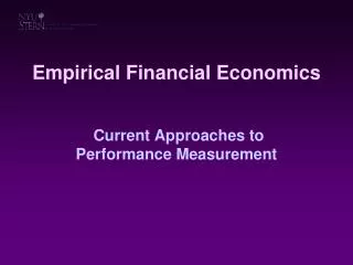
Empirical Financial Economics. 5. Current Approaches to Performance Measurement. Stephen Brown NYU Stern School of Business UNSW PhD Seminar, June 19-21 2006. Overview of lecture. Standard approaches Theoretical foundation Practical implementation Relation to style analysis

E N D
Empirical Financial Economics 5. Current Approaches to Performance Measurement Stephen Brown NYU Stern School of Business UNSW PhD Seminar, June 19-21 2006
Overview of lecture • Standard approaches • Theoretical foundation • Practical implementation • Relation to style analysis • Gaming performance metrics
Performance measurement Style: Index Arbitrage, 100% in cash at close of trading
Universe Comparisons 40% Brownian Management 35% S&P 500 30% 25% 20% 15% 10% 5% 1 Year 3 Years 5 Years One Quarter Periods ending Dec 31 2002
Total Return comparison Average Return A B C D
Total Return comparison Average Return A Manager A best RS&P = 13.68% S&P 500 B C Manager D worst D rf = 1.08% Treasury Bills
Total Return comparison Average Return A B C D
Sharpe ratio comparison Average Return A B C D Standard Deviation
Sharpe ratio comparison Average Return A RS&P = 13.68% S&P 500 B C D rf = 1.08% Treasury Bills Standard Deviation ^ σS&P = 20.0%
Sharpe ratio comparison Average Return A RS&P = 13.68% S&P 500 B C Manager C worst Sharpe ratio = D Manager D best Average return – rf Standard Deviation rf = 1.08% Treasury Bills Standard Deviation ^ σS&P = 20.0%
Sharpe ratio comparison Average Return A RS&P = 13.68% S&P 500 B C D rf = 1.08% Treasury Bills Standard Deviation ^ σS&P = 20.0%
Jensen’s Alpha comparison Average Return A RS&P = 13.68% S&P 500 B Manager B worst C Manager C best Jensen’s alpha = D Average return – {rf + β (RS&P - rf )} rf = 1.08% Treasury Bills Beta βS&P = 1.0
Intertemporal equilibrium model • Multiperiod problem: • First order conditions: • Stochastic discount factor interpretation: • “stochastic discount factor”, “pricing kernel”
Value of Private Information • Investor has access to information • Value of is given by where and are returns on optimal portfolios given and • Under CAPM (Chen & Knez 1996) • Jensen’s alpha measures value of private information
The geometry of mean variance Note: returns are in excess of the risk free rate
Informed portfolio strategy • Excess return on informed strategy where is the return on an optimal orthogonal portfolio (MacKinlay 1995) • Sharpe ratio squared of informed strategy • Assumes well diversified portfolios
Informed portfolio strategy • Excess return on informed strategy where is the return on an optimal orthogonal portfolio (MacKinlay 1995) • Sharpe ratio squared of informed strategy • Assumes well diversified portfolios Used in tests of mean variance efficiency of benchmark
Practical issues • Sharpe ratio sensitive to diversification, but invariant to leverage • Risk premium and standard deviation proportionate to fraction of investment financed by borrowing • Jensen’s alpha invariant to diversification, but sensitive to leverage • In a complete market impliesthrough borrowing (Goetzmann et al 2002)
Changes in Information Set • How do we measure alpha when information set is not constant? • Rolling regression, use subperiods to estimate (not subscript) – Sharpe (1992) • Use macroeconomic variable controls – Ferson and Schadt(1996) • Use GSC procedure – Brown and Goetzmann (1997)
Style management is crucial … Economist, July 16, 1995 But who determines styles?
Characteristics-based Styles • Traditional approach … • are changing characteristics (PER, Price/Book) • are returns to characteristics • Style benchmarks are given by
Returns-based Styles • Sharpe (1992) approach … • are a dynamic portfolio strategy • are benchmark portfolio returns • Style benchmarks are given by
Returns-based Styles • GSC (1997) approach … • vary through time but are fixed for style • Allocate funds to styles directly using • Style benchmarks are given by
Concave payout strategies • Zero net investment overlay strategy (Weisman 2002) • Uses only public information • Designed to yield Sharpe ratio greater than benchmark • Using strategies that are concave to benchmark
Concave payout strategies • Zero net investment overlay strategy (Weisman 2002) • Uses only public information • Designed to yield Sharpe ratio greater than benchmark • Using strategies that are concave to benchmark • Why should we care? • Sharpe ratio obviously inappropriate here • But is metric of choice of hedge funds and derivatives traders
We should care! • Delegated fund management • Fund flow, compensation based on historical performance • Limited incentive to monitor high Sharpe ratios • Behavioral issues • Prospect theory: lock in gains, gamble on loss • Are there incentives to control this behavior?
Sharpe Ratio of Benchmark Sharpe ratio = .631
Maximum Sharpe Ratio Sharpe ratio = .748
Examples of concave payout strategies • Long-term asset mix guidelines
Examples of concave payout strategies • Unhedged short volatility • Writing out of the money calls and puts
Examples of concave payout strategies • Loss averse trading • a.k.a. “Doubling”
Examples of concave payout strategies • Long-term asset mix guidelines • Unhedged short volatility • Writing out of the money calls and puts • Loss averse trading • a.k.a. “Doubling”
Forensic Finance • Implications of concave payoff strategies • Patterns of returns
Forensic Finance • Implications of Informationless investing • Patterns of returns • are returns concave to benchmark?
Forensic Finance • Implications of concave payoff strategies • Patterns of returns • are returns concave to benchmark? • Patterns of security holdings
Forensic Finance • Implications of concave payoff strategies • Patterns of returns • are returns concave to benchmark? • Patterns of security holdings • do security holdings produce concave payouts?
Forensic Finance • Implications of concave payoff strategies • Patterns of returns • are returns concave to benchmark? • Patterns of security holdings • do security holdings produce concave payouts? • Patterns of trading
Forensic Finance • Implications of concave payoff strategies • Patterns of returns • are returns concave to benchmark? • Patterns of security holdings • do security holdings produce concave payouts? • Patterns of trading • does pattern of trading lead to concave payouts?