Download
1 / 15
150 likes | 261 Vues
This document focuses on the preparation of nonnumerical (alpha) variables for data mining. Key methods are discussed, including remapping techniques such as one-of-n and m-of-n approaches, which convert categorical data into numerical formats. The paper details the advantages and disadvantages of these methods, highlights challenges with ill-formed problems, and explores the implications of ordering in data. It emphasizes the importance of proper state space management and offers insights into how geographical or characteristic divisions can create useful pseudo-variables.

E N D
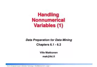
Handling Nonnumerical Variables (1) Data Preparation for Data Mining Chapters 6.1 - 6.2 Ville Makkonen mak@iki.fi
Contents Remapping • One-of-n • m-of-n • Ordering • Ill-formed problems (one-to-many patterns) • Circular discontinuity State Space • Basic properties • Locations and points • Density • Topography • Phase space • Mapping alphas
Remapping overview • Nonnumerical (alpha) variables are remapped to numerical values • numerical to numerical remapping is of course also possible • The form of remapping depends on the modeling tool used • Remapping can be useful if: • a remapped pseudo-variable will have a high information density • dimensionality is only slightly increased • some form of reasoning can be given for remapping • model requires that no ordering of alphas is used
One-of-n Remapping • One binary pseudo-variable per alpha label • Only a single variable "on" for each sample • Advantages: • mean of each pseudo-variable is directly proportional to the number of corresponding labels in the sample • useful in prediction • Disadvantages: • big increase in dimensionality • low pseudo-variable density • in prediction, many pseudo-variables will be on for a single output • Example: • one variable for each European country FIN GER ITA POL ... Finland 1 Germany 1 Italy 1 Poland 1 ...
m-of-n Remapping • Pseudo variables created from alpha label characteristics • Several pseudo-variables "on" per sample • Advantages: • dimensionality increased less than with one-to-n (if less pseudo-variables than labels) • useful new information possibly added • Disadvantages: • highly dependent on domain knowledge • Example: • countries are divided according to geographic location, population, GNP, etc. North Centr South East Big Rich ... Finland 1 1 1 Germany 1 1 1 Italy 1 1 1 Poland 1 1 1 ...
Ordering • If the alpha labels to be remapped contain an implicit ordering, it should be preserved • Example: labels for lengths of time, sizes etc. • Remapping can be used to ascertain that there is no implication of ordering
1.6 1.4 1.2 • Same profit curve, axes reversed: x = profit, y = price 1 0.8 • MATLAB POLYFIT result(good) • MATLAB POLYFIT result(bad) 0.6 0.4 0.9 0.2 0.8 0 0.7 -0.2 0 0.1 0.2 0.3 0.4 0.5 0.6 0.7 0.8 0.9 1 0.6 0.5 0.4 0.3 0.2 0.1 0 0 0.1 0.2 0.3 0.4 0.5 0.6 0.7 0.8 0.9 1 Ill-formed Problems • The one-to-many pattern: several input values indicate the same output • Modeling tools that try to find a function fitting the data fail • Profit curve: x = price, y = profit
Remapping Ill-formed Problems • Areas of multivalued output hard to detect, easiest in data survey • If one-to-many situation is known, easiest to correct by data preparation • Additional information (more dimensions) must be added to distinguish between the situations of identical output • Other ways to correct one-to-may problem mentioned: • "Reverse the axes" - reflect the data in an appropriate state space • Use a local distortion to "untwist" • Risky • Use modeling that can deal with one-to-many
Better labeling: weeks start from 0 in January, rise to 1 in June, then decrease back to 0. 0.25 : 0.75 0 Jan : 0.25 0.25 • The week number indicator is called lead variable. In addition a lag variable is used to indicate the lead variable value quarter of a year ago. • Two variables are needed to be able to unambiguously define the time (two dimensions - two coordinates) Jun 1 0.75 : 0.25 Remapping Circular Discontinuity • Annual cycles: months, days of month, weeks … • Also other cycles: weeks to a chosen annual event • Discontinuity in labeling (from 12 to 1, 31 to 1, 52 to 1), prevents most modeling tools from finding cyclical information 0.75 : 0.75
State Space Overview • N-dimensional space, variables of the data set as dimensions • Variable ranges limited, often normalized to unit state space • modeling tools cannot cope with monotonicity • Each point represents a particular state of the system • Distances between points calculated with Pythagorean theorem • d2 = Σ (d12 + d22 + … + dn2) • distance increases as number of dimensions (n) increase • measured distance can be normalized in unit state space, since dmax2 = n • Points close together are called neighbors • Neighboring states are more likely to share common features • Nature of neighborhoods may change from place to place
Locations, points and density • Location or position indicates specific place in state space • Point or data point indicates a location which represents a measured system state • Density measured as number of points in specific volume • State space volume is fixed, but number of points depends on the size of the data set • Relative density most useful to examine • Relative density = specific area density / mean density • Unaffected by changing data set size • Not usually normalized
By distance to n nearest neigbors • value of n? • closest neighbors may be "biased" to one direction • better estimate when area divided and nearest neighbor found in each division Estimating density • By number of points in an area (volume) • depends on shape of area • rotation and translation affect result
State space topography • Values can be smoothed between the points to get a continuous density gradient • Density values can be represented as height on the map (high density down, low density up) • (seems illogical - why not vice versa?) • Contours of constant "elevation" can be drawn • Contours point out natural clusters in the data - the valleys of high density • Data points can be thought to form geometric objects • higher-dimensional objects can be projected ("cast shadows") to a lower-dimensional space
Phase space and mapping alphas • Phase space is used to represent features of objects or systems other than their state • Alpha labels are positioned into phase space each with specific distance and direction from neigboring labels • Once the appropriate places for the labels (in phase space) are known, the appropriate label values (in state space) can be found • The alpha labels are associated with some particular area on the state space map • There is no absolute value associated with each label, but the order and distance of labels is preserved in the numeration
Examples with Montreal Canadiens • Example 1 • two-dimensional state space consisting of player height and weight • arbitrary labels are assigned for player weights • the labels are given values according to the normalized height of the player • the correlation of original and recovered weights is quite good (0.85), which indicates that taller hockey players tend also to weigh more than short ones • Example 2 • three-dimensional state space consisting of player height, weight and position • player positions (defense, forward, goal, reserve) are inherently labeled • the labels are given (two-dimensional) values by calculating the mean height and weight of all players represented by that label • the labels fall nearly on a straight line in (height-weight) state space, so a single numerical label (which represents the normalized position on the line) is sufficient