Download

1 / 41
430 likes | 737 Vues
In the name of God. Determining the Size of a Sample. Dr Mohammad Hossein Fallahzade . Sample Accuracy. Sample accuracy: refers to how close a random sample’s statistic is to the true population’s value it represents Important points: Sample size is not related to representativeness

E N D
In the name of God Determining the Size of a Sample Dr Mohammad Hossein Fallahzade
Sample Accuracy • Sample accuracy:refers to how close a random sample’s statistic is to the true population’s value it represents • Important points: • Sample size is not related to representativeness • Sample size is related to accuracy
Sample Size and Accuracy • Intuition: Which is more accurate: a large probability sample or a small probability sample? • The larger a probability sample is, the more accurate it is (less sample error).
± n 550 - 2000 = 1,450 4% - 2% = ±2% Probability sample accuracy (error) can be calculated with a simple formula, and expressed as a ± % number.
Sample Size Formula • Fortunately, statisticians have given us a formula which is based upon these relationships. • The formula requires that we • Specify the amount of confidence we wish • Estimate the variance in the population • Specify the amount of desired accuracy we want. • When we specify the above, the formula tells us what sample we need to use…n
Sample Size and Population Size • Where is N (size of the population) in the sample size determination formula? In almost all cases, the accuracy (sample error) of a probability sample is independent of the size of the population.
Sample Size Formula • Standard sample size formula for estimating a percentage:
Practical Considerations in Sample Size Determination • How to estimate variability (p times q) in the population • Expect the worst cast (p=50; q=50) • Estimate variability: Previous studies? Conduct a pilot study?
Practical Considerations in Sample Size Determination • How to determine the amount of desired sample error • Convention is + or – 5% • The more important the decision, the more (smaller number) the sample error.
Practical Considerations in Sample Size Determination • How to decide on the level of confidence desired • The more confidence, the larger the sample size. • Convention is 95% (z=1.96) • The more important the decision, the more likely the manager will want more confidence. 99% confidence, z=2.58.
ExampleEstimating a Percentage in the Population • What is the required sample size? • Five years ago a survey showed that 42% of consumers were aware of the company’s brand (Consumers were either “aware” or “not aware”) • After an intense ad campaign, management wants to conduct another survey and they want to be 95% confident that the survey estimate will be within ±5% of the true percentage of “aware” consumers in the population. • What is n?
Estimating a Percentage: What is n? • Z=1.96 (95% confidence) • p=42 • q=100-p=58 • e=5 • What is n?
Estimating a Mean • Estimating a mean requires a different formula (See MRI 13.2, p. 378) • Z is determined the same way (1.96 or 2.58) • E is expressed in terms of the units we are estimating (i.e., if we are measuring attitudes on a 1-7 scale, we may want error to be no more than ± .5 scale units • S is a little more difficult to estimate…
Estimating s • Since we are estimating a mean, we can assume that our data are either interval or ratio. When we have interval or ratio data, the standard deviation, s, may be used as a measure of variance.
Estimating s • How to estimate s? • Use standard deviation from a previous study on the target population. • Conduct a pilot study of a few members of the target population and calculate s. • Estimate the range the value you are estimating can take on (minimum and maximum value) and divide the range by 6.
Estimating s • Why divide the range by 6? • The range covers the entire distribution and ± 3 (or 6) standard deviations cover 99.9% of the area under the normal curve. Since we are estimating one standard deviation, we divide the range by 6.
Practice Example • A client wants to survey out-shopping intentions (percentage of people saying “yes” to a question regarding their intentions to out-shop) among heads of households in Antigonish. The client wants a ± 3%, 19 times out of 20. There are 3,000 households in the catchment area. What sample size should be used?
Sample size Considerations Needed for Two Independent Groups
7 ingredients for sample size calculations • Research question to be answered • Outcome measure • Effect size • Variability & success proportions • For continuous outcome • For binary outcome • Type I error • Type II error • Other factors
Further explanations of ingredient 1 • Research question to be answered • Translate the question into a clear hypothesis! • For example, • H0: there is no difference between treatment and control • H1: there are differences between treatment and control • Hypothesis Statistical results Conclusion • statistically significant result (that is, p<0.05) • enough evidence to reject H0 accept H1 • statistically non-significant result (that is, p>0.05) • no evidence to reject H0
Further explanations of ingredient 2 • Outcome measures • Should only have one primary outcome measure per study! • Could have a secondary outcome measure, but we can only sample sizing/powering for the primary outcome • May not have enough power for any results relating to the secondary outcome • Recall the two types of variables: • Continuous • Categorical • If the variable has 2 categories Binary
Further explanations of ingredient 3 • Effect Size (d) – from the word ‘difference’ • The magnitude of difference that we are looking for • Clinically important difference • For 2 treatment arms: • difference in means if continuous outcome • difference in success proportions if binary outcome • Minimum value worth detecting • Decide what the minimum ‘better’ means by looking at the endpoint and by considering background noise • Headache? or Moderate & severe headache? or Migraine? • Values could be found in previous literatures if they were doing similar study or can be estimated base on clinical experience but make sure it is reasonable (Remember GIGO!)
Further explanations of ingredient 3… • Effect Size (d) • Example: In previous study, morbidity of a certain illness under conventional care is known to be 73% • Interested in reducing morbidity to 50% (clinically important) • Therefore the effect size is 23% • A difference between these morbidities • Example:Summarising all the studies with similar setting and characteristics regarding to a specific outcome measure, e.g. pain relief • The overall response rate on Placebo is 32% • The overall response rate on Active is 50% • The overall estimate of the difference between Active and Placebo is 18% • Of all the differences that are found in these studies, the smallest difference observed is 12% • Could be the minimum value worth detecting
Further explanations of ingredient 4.1 Variability (σ) – pronounce as Sigma • For continuous outcome only! • Standard deviation (σ) or variance (σ2) represents the spread of the distribution of a continuous variable • Values can usually be found in previous literatures or can be estimated base on clinical experience but make sure it is reasonable (GIGO!)
Pooled standard deviation If there are several studies with variance estimates available it is recommended that an overall estimate of the population variance or the pooled variance estimates, σp2, is obtained from the following formula where k is the number of studies, σi2 is the variance estimate from the ith study and dfi is the degrees of freedom about this variance (which is the corresponding number of observations in the group minus 1, i.e. (ni - 1)).
Pooled standard deviation… Example: The following descriptive statistics (number of subjects, mean ± standard deviation) of an outcome measure for each treatment arm were reported, Treatment A: nA = 83, meanA±σA = 40.98 ± 22.52 Treatment B: nB = 87, meanB±σB = 37.89 ± 19.74 Using the formula above, the pooled variance (σp2) and the pooled SD (σp) is
Further explanations of ingredient 4.2 Success proportions (p) • For binary outcome only! • Normally concerning Cured/Not Cured, Alive/Dead…etc • Require to know the success proportion of the binary outcome for each group or treatment arm first, can be found in previous literatures or estimate with clinical experience • In the above table, suppose we are interested in the proportion of Alive, then the success proportions in each treatment are pA and pB for treatment A and B respectively • Denote is the average success proportion, i.e. (pA + pB)/2 • We can use these information to find out the effect size and the standard deviation • The effect size is the difference of the two success proportions, i.e. pA - pB • The estimated standard deviation is , where is between 0 and 100
Further explanations of ingredients 5 & 6 Type I error (α) & Type II error (β) • You should have heard these mentioned in the Hypothesis Testing session, hence this is just a reminder • Due to the fact that we are sampling from a population • Uncertainty is introduced • Quality of the sample will have an impact on our conclusion • Error does exist • There are two types of error: • Type I error (α): observed something in our sample but not exist in the population (the truth) • e.g. drinking water leads to cancer • Type II error (β): observed nothing in our sample but something exist in the population (the truth) • e.g. smoking doesn’t lead to cancer
Further explanations of ingredients 5 & 6… Type I error (α) & Type II error (β) • Type I error (α): usually allow for 5% • Significant level = α cut-off point for p-value, i.e. 0.05
Further explanations of ingredients 5 & 6… Type I error (α) & Type II error (β) • Type II error (β): usually allow for 10% or 20%, more than Type I error (since Type I error is referred as society risk and hence more crucial to pharmaceutical company financially) • Power of the study = 1-Type II error = 1-β, usually use 80% or 90%, the probability of detecting a difference in our study if there is one in the whole population
Further explanations of ingredient 7 Other factors • Calculated sample size meaning the number of subjects required during the analysis, not the number to start with for recruiting subjects, if you want to detect a certain effect size with a specific significance and power • Study design: • Response rate: data gathering affect the response rate, e.g. about 50% response rate by postal questionnaire • Drop-out rate: due to following subjects for a long period of time, e.g. cohort study, usually 20% - 25% • Can increase the sample size by a suitable percentage to allow for these problems • for example, increase calculated sample size (n) by 25%
Formula for 2 independent groups • From the 7 ingredients, there are 4 crucial factors involve in the actual sample size calculation • Effect size (d): the size of the difference we want to be able to detect • Variability (σ) or ( ): the standard deviation of the continuous outcome or the estimation for the binary outcome • Level of significance (α): the risk of a Type I error we will accept • Power (1-β): the risk of a Type II error we will accept
Formula for 2 independent groups… • We use these 4 factors to generalise a formula to calculate sample size for 2 groups with continuous or binary outcome • The formula is: • where is the standardised effect size • i.e. effect size / variability • = d/ for continuous outcome • = for binary outcome
What is z-score? Z-score is the number of standard deviations above/below the mean. z = (x – )/ z-score
What is z(1-/2) and z(1-)? • z(1-/2)is a value from the Normal distribution relating to significance level • If the level of significance is set to 5%, then = 0.05 • For 2-sided test, z(1-/2)= z0.975 = 1.9600 • If the level of significance is set to 1%, then = 0.01 • For 2-sided test, z(1-/2)= z0.995 = 2.5758 • z(1-)is a value from the Normal distribution relating to power • If is set to 10%, then the power is 90%, so 1- = 0.90 • For 1-sided test, z(1-)= z0.90 = 1.2816 • If is set to 20%, then the power is 80%, so 1- = 0.80 • For 1-sided test, z(1-)= z0.80 = 0.8416
Table of z-scores z-score
The quick formula • We can pre-calculate [z(1-/2)+ z(1-)]2, and call this k, using the relevant z-scores provided in the table from the previous slide for different combination of level of significance and power 1-, the formula then becomes n (per group) = 2k/2 • Remember to multiply the calculated sample size (n) by 2 to allow for 2 groups! • Always round up your final sample size where is effect size / variability = d/ for continuous outcome = for binary outcome
Even simpler! • For 5% significance level and power of 80% n = 2 (2 7.85)/2 32/2 (Total for 2 groups) • For 1% significance level and power of 90% n = 2 (2 11.68)/2 60/2 (Total for 2 groups) “A sample size of n within two groups will have 80% (and 90% respectively) power to detect the standardised effect size , and that the test will be performed at the 5% (and 1% respectively) significance level (two-sided).” Note that =/, hence the required sample size increases as increases, or as decreases.
The 4 factors & sample size • Referring to the quick formula, we can predict the effect on the sample size if we increase/decrease the value of each of the 4 factors • If the level of significance () decrease, e.g. from 5% to 1% • sample size increase • If Type II error rate () decrease, power (1- ) increase, e.g. from 80% to 90% • sample size increase • If the effect size (d) decrease, e.g. detecting a smaller difference between the 2 groups • sample size increase • If the variability () decrease, e.g. assuming the outcome measure has a smaller spread or less vary • sample size decrease
…with continuous outcome Example: Differences between means In a trial to compare the effects of two oral contraceptives on blood pressure (over one year), it is anticipated that one drug will increase diastolic blood pressure by 3mmHg, and the other will not change it. The standard deviation (of the changes in blood pressure) in both groups is expected to be 10mmHg. How many patients are required for this difference to be significant at the 5% level (with 80% power)? women per group and a total of 350 women need to be recruited.
…with binary outcome Example: Difference between proportions In a randomised clinical trial, the placebo response is anticipated to be 25%, and the active treatment response 65%. How many patients are needed if a two-sided test at the 1% level is planned, and a power of 90% is required? so n=47 per group and a total of 94 patients are needed for this study.