Download
1 / 18
180 likes | 407 Vues
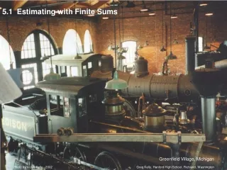
5.1 Estimating with Finite Sums. Distance Traveled The distance traveled and the area are both found by multiplying the rate by the change in time.

E N D
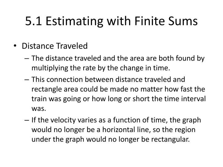
5.1 Estimating with Finite Sums • Distance Traveled • The distance traveled and the area are both found by multiplying the rate by the change in time. • This connection between distance traveled and rectangle area could be made no matter how fast the train was going or how long or short the time interval was. • If the velocity varies as a function of time, the graph would no longer be a horizontal line, so the region under the graph would no longer be rectangular.
Distance Traveled • Would the area of this irregular region still give the total distance traveled over the time interval? • Newton and Leibniz (and other mathematicians) considered this question. They thought that it would and that is why they were interested in a calculus for finding areas under curves. • They argued that, just as the total area could be formed by summing the areas of the (essentially rectangular) strips, the total distance traveled could be found by summing the small distances traveled over the tiny time intervals.
Finding Distance Traveled when Velocity Varies • A particle starts at x = 0 and moves along the x-axis with velocity v(t) = t² for time t ≥ 0. Where is the particle at t = 3? • We graph v and partition the time interval [0 , 3] into subintervals of length Δt.
Finding Distance Traveled when Velocity Varies • Notice that the region under the curve is partitioned into thin strips with bases of length ¼ and curved tops that slope upward from left to right. • Might not know how to find the area of each strip, but you can get a good approximation of it by finding the area of a suitable rectangle.
Finding Distance Traveled when Velocity Varies • We use the rectangle whose height is the y-coordinate of the function at the midpoint of its base. • The area of this narrow rectangle approximates the distance traveled over the time subinterval. • Adding all the areas (distances) gives an approximation of the total area under the curve (total distance traveled) from t = 0 to t = 3.
Finding Distance Traveled when Velocity Varies • Computing this sum of areas is straightforward. Each rectangle has a base of length Δ t = ¼, while the height of each rectangle can be found by evaluating the function at the midpoint of the interval.
Finding Distance Traveled when Velocity Varies • We derive the area (1/4)(mi)² for each of the twelve subintervals and add them: • Since this number approximates the area and the total distance traveled by the particle, we conclude that the particle has moved approximately 9 units in 3 seconds. If it starts at x = 0, then it is very close to x = 0 when t = 3.
Rectangular Approximation Method (RAM) • In Example 1, we used the Midpoint Rectangular Approximation Method (MRAM) to approximate the area under the curve. • The name suggests the choice we made when determining the heights of the approximating rectangles: • We evaluated the function at the midpoint of each subinterval. • If instead we had evaluated the function at the left-hand endpoints we would have obtained the LRAM approximation, and if we had used the right-hand endpoints we would have obtained the RRAM approximation.
Estimating Area Under the Graph of a Nonnegative Function • Figure 5.8 shows the graph of f(x) = x2 sin x on the interval [0 , 3]. Estimate the area under the curve from x = 0 to x = 3.
Estimating Area Under the Graph of a Nonnegative Function • Figure 5.8 shows the graph of f(x) = x2 sin x on the interval [0 , 3]. Estimate the area under the curve from x = 0 to x = 3. • It is not necessary to compute all three sums each time just to approximate the area, but we wanted to show again how all three sums approach the same number. With 1000 subintervals, all three agree in the first three digits. (The exact area is -7 cos 3 + 6 sin 3 – 2 which is 5.77666752456 to twelve digits.
Estimating the Volume of a Sphere • See Example 3 on p. 267.
Cardiac Output • The number of liters of blood your heart pumps in a fixed time interval is called your cardiac output.
Computing Cardiac Output from Dye Concentration • Estimate the cardiac output of the patient whose data appear in Table 5.2 and Figure 5.10. Give the estimate in liters per minute.
Computing Cardiac Output from Dye Concentration • Estimate the cardiac output of the patient whose data appear in Table 5.2 and Figure 5.10. Give the estimate in liters per minute.