Lecture 2 and 3 - Dimensional Modelling

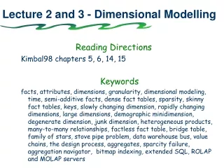
1. Lecture 2 and 3 - Dimensional Modelling Reading Directions Kimbal98 chapters 5, 6, 14, 15 Keywords facts, attributes, dimensions, granularity, dimensional modeling, time, semi-additive facts, dense fact tables, sparsity, skinny fact tables, keys, slowly changing dimension, rapidly changing dimensions, large dimensions, demographic minidimension, degenerate dimension, junk dimension, heterogeneous products, many-to-many relationships, factless fact table, bridge table, family of stars, stove pipe problem, data warehouse bus, value chains, the design process, aggregates, sparcity failure, aggregation navigator, bitmap indexing, extended SQL, ROLAP and MOLAP servers

2. OLTP vs. OLAP holds current data stores detailed data data is dynamic repetitive processing high level of transaction throughput predictable pattern of usage transaction driven application oriented support day-to-day decisions serves large number of operational users holds historic data stores detailed and summarised data data is largely static ad-hoc, unstructured and heuristic processing medium or low-level of transaction throughput unpredictable pattern of usage analysis driven subject oriented supports strategic decisions serves relatively lower level of managerial users

3. Some basic concepts • Fact • “something not known in advance”, • an observation • many facts (but not all) have numerical, continuously values e.g., the price of a product, quantity • Attribute • “describe a characteristic of a tangible thing” • “we do not measure them, we usually know them” • usually text fields, with discrete values e.g., the flavour of a product, the size of a product

4. Some basic concepts 2 • Dimension • a business perspective from which data is looked upon • “a collection of text like attributes that are highly correlated” e.g. Product, Store, Time • Granularity • the level of detail of data contained in the data warehouse e.g. Daily item totals by product, by store

5. Example of a Dimensional Model

6. The Time Dimension

7. The Standard Template Query SELECT p.brand, sum(f.dollar), sum(f.units) FROM salesfact f, product p, time t WHERE f.prductkey = p.productkey AND f.timekey = t.timekey AND t.quarter = ’1Q1995’ GROUP BY p.brand ORDER BY p.brand

8. An Example Answer Set Aggregated fact Row header

9. Facts • (Perfectly) Additive • a fact is additive if it is possible to add it across all the dimensions e.g., discrete numerical measures of activity, i.e., quantity sold, dollars soled • Semiadditive • a fact is semiadditive if it is possible to add it along only some of the dimensions e.g., numerical measures of intensity, i.e., account balance, inventory level • Non-additive • facts that can not be added at all e.g.,

10. Facts and the Additive Property 28/3, paper1, store1, 25, 250, 20 28/3, paper2, store1, 35, 350, 30 60, 600 28/3, paper, store1, 25, 250, 20 28/3, paper, store2, 35, 350, 30 60, 600, 50 28/3, paper, store1, 25, 250, 20 29/3, paper, store1, 35, 350, 30 60, 600, 50

11. Semiadditive fact - example NB! customer_count is not additive across the product dimension 28/3, tissue paper, store1, 25, 250, 20 28/3, paper towels, store1, 35, 350, 30 ---- 50 Is the number of customers who bought either paper towels or tissue paper 50? No, the number could be anywhere between 30 and 50.

12. Numerical Measures of Intensity • All measures that record a static level, such as account balance and inventory level, are non-additive across time. • However, these measures may be usefully aggregated across time by averaging over the number of time periods. • Note that, the SQL AVG can not be used for this. • What is the average daily inventory of a brand in a geographic region during a given week? • Let the brand cluster 3 products, the region has 4 stores, and we have 7 days/week. • Using the SQL AVG would divide the summed value into 3*4*7=84 • The correct answer is to divide the summed inventory value by 7

13. Sparsity • The matrices, represented by multidimensional models are often 99% sparse. • Sparsity is dealt with by simply not creatingrecords for the cells that are not filled in the matrix. If nothing has happened no record is created. • Pre-aggregation and storage of aggregates can however lead to sparsity failure which places large demands on data storage

14. Skinny fact tables • As the fact table contains the vast volume of records it is important that it is memory space efficient • Foreign keys are usually represented in integer form and do not require much memory space • Facts too are often numeric properties and can usually be represented as integers (contrast to dimensional attributes which are usually long text strings) • This space efficiency is critical to the memory space consumption of the data warehouse

15. Keys • Choice the data warehouse keys to be meaningless surrogate keys • Let a surrogate key be a simple integer • 4-byte (--------,--------,--------,--------) can contain 232 values (> 2 billion positive integers, starting with 1)

16. Keys • Use surrogate keys also for the Time dimension • SQL-based date key, is typically 8 bytes, so 4 bytes are wasted • bypassing joins leads to embedding knowledge of the calendar in the application, rather than reading it from the time dimension • it is not possible to encode a data stamp as “I do not know”, “It has not happen yet”, etc • Avoid smart keys • Avoid production keys

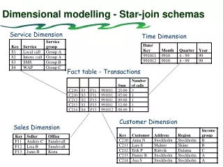
17. Dimensional modelling - Star-join schemas Service Dimension Time Dimension Fact table - Transactions Number Sum of calls C210 S1 F11 991011 25:00 3 C210 S3 F11 991011 05:00 1 C212 S2 F13 991011 89:00 1 C213 S1 F13 991011 12:00 1 C214 S4 F13 991012 08:00 1 Customer Dimension Sales Dimension

18. Slowly Changing Dimensions • Type 1: Overwrite the dimension record with the new values, thereby losing history • Type 2: Create a new additional dimension record using a new value of the surrogate key • Type 3: Create a new field in the dimension record to store the new value of the attribute For example, the product or customer dimension The assumption: the key does not change, but some of the attributes does.

19. Type 1 Overwrite the old value of an attribute with a new one e.g. + easy to implement - avoids the real goal, which is to accurately track history

20. Type 2 Create a new additional dimension record • A generalised (surrogate) key is required (which is a responsibility of the data warehouse team) Fact table Dimension table

21. Type 3 Create a new field in the dimension record

22. Rapidly Changing Dimensions From the previous slides: What is slow? What if the changes are fast? Must a different design technique be used? • Small dimensions: • the same technologies as for slowly changing dimensions may be applied • Large dimensions: • the choice of indexing techniques and data design approaches are important • find suppress duplicate entries in the dimension • do not create additional records to handle the slowly changing dimension problem

23. Rapidly changing very large dimensions • Break off some of the attributes into their own separate dimension(s), a demographic dimension(s). • force the attributes selected to the demographic dimension to have relatively small number of discrete values • build upp the demographic dimension with all possible discrete attributes combinations • construct a surrogate demographic key for this dimension NB! The demographic attributes are the one of the heavily used attributes. Their values are often compared in order to identify interesting subsets.

24. Demographic Minidimension

25. Demographic Minidimension Three values Two values 3*2*2=12 rows Two values

26. Two Demographic Minidimensions

27. Demographic Minidimension • Advantages • frequent ‘snapshoting’ of customers profiles with no increase in data storage or data complexity • Drawbacks • the demographic attributes are clumped into banded ranges of discrete values (it is impractical to change the set of value bands at a later time) • the demographic dimension itself can not be allowed to grow too large • slower down the browsing

28. Degenerate Dimension • A degenerate dimension is represented by a dimension key attribute(s) with no corresponding dimension table • Occurs usually in line-item oriented fact table design

29. Junk Dimensions • Leaving the flags and attributes unchanged in the fact table record • Making each flag and attribute into its own separate dimension • Stripping out all of these flags and attributes from the design When a number of miscellaneous flags and text attributes exist, the following design alternatives should be avoided: A better alternative is to create a junk dimension. A junk dimension is a convenient grouping of flags and attributes to get them out of a fact table into a useful dimensional framework

30. Heterogeneous Products Some products have many, many distinguishing attributes and many possible permutations (usually on the basis of some customised offer). This results in immense product dimensions and bad browsing performance • In order to deal with this, fact tables with accompanying product dimensions can be created for each product type - these are known as custom fact tables • Primary core facts on the products types are kept in a core fact table • The core facts are copied in each of the customer fact tables

31. Heterogeneous Products

32. Heterogeneous Products

33. Dealing with many-to-many relationships • Many to many relationships (M-to-M) between entities (tables) are difficult to deal with in a any database design situation. E.g. A customer can have many accounts and an account can have many customers • A new table can be created to capture the relationship between the tables • Many to many relations between dimensional tables in a star-join schema can be handle by creating a factless fact table or a bridge table

34. Factless fact tables • Some fact tables quite simply have no measured facts! • Are useful to describe events and coverage, i.e. the tables contain information that something has happened. • Often used to represent many-to-many relationships • The only thing they contain is a concatenated key, they do still however represent a focal event which is identified by the combination of conditions referenced in the dimension tables • There are two main types of factless fact tables: • event tracking tables • coverage tables

35. Factless fact tables Event tracking tables - records events, e.g. records every time a student attends a course, or people involved in accidents and vehicles involved in accidents Coverage tables - description of of something that did not happend, e.g. which product did not sell during a promotion campaign.

36. Bridge table Problem: There are multiple diagnosis involved in the billed amount? The users of the dw want to know for how much money a certain diagnosis is billed for?

37. Bridge table • Handle open ended many-value attribute, i.e dimensions with many values which are not knowable before the fact table is created • A weighting factor in the bridge table to add up the billed amount correctly for each diagnosis

38. Partitioning strategy • for performace-related and manageablity reasons • usually for handling the fact table Horisontal partitioning - speed up queries by minimising the data to be scanned (without using an index) - partition by time most common Vertical partitioning - data is split vertically - two forms: normalisation and row splitting - consider row splitting if some columns are access infrequently Dim Fact Dim Dim

39. A family of stars

40. A family of stars • A dimensional model of a data warehouse for a large data warehouse consists of between 10 and 25 similar-looking star-join schemas. Each star join will have 5 to 15 dimensional tables. • Conformed (shared) dimensions for drill-across. A Conformed dimension is a dimension that means the same thing with every possible fact table to which it can be joined.

41. The stove pipe problem IT system5 IT- system4 IT- system3 IT- system2 IT- system1 Market Purchase Production Shipment Service Business process

42. The stove pipe problem IT system5 IT- system4 IT- system3 IT- system2 IT- system1 IT systems Market Purchase Production Shipment Service Business process

43. Problems of Data Warehousing • Complexity of integration • Hidden problems with source systems • Data homogenisation • Underestimation of resources for data loading • Required data not captured • High maintenance • Long duration projects • Why not integrating the legacy applications (OLTP systems) instead?

44. The Data Warehouse Bus Orders Production Dimensions Time Sales Rep Customer Promotion Product Plant Distr. Center

45. Value chains as families of star-join schemas • There are two sides to the value chain • the demand side- the steps needed to satisfy the customers’ demand for the product • the supply side - the steps needed to manufacture the products from original ingredients or parts • The chain consists of a sequence of inventory and flow star-join schemata • joining the different star-join schemata is only possible when two sequential schemata have a common, identical dimension • Sometimes the represented chain can be extended beyond the bounds of the business itself

46. Supply Chain Row material production Ingredient purchasing Ingredient delivery Ingredient inventory Bill of materials Manufacturing process control Manufacturing costs Packaging Trans-shipping to warehouse Finished goods inventory Demand Chain Finished goods inventory Manufacturing shipments Distributor inventory Distributor shipments Retail inventory Retail sales Value chains as families of star-join schemas

47. Dimensional modelling vs. ER-modelling Entity-relationship modelling - a logical design technique to eliminate data redundancy to keep consistency and storage efficiency - makes transaction simple and deterministic - ER models for enterprise are usually complex, e.g. they often have hundreds, or even thousands, of entities/tables Dimensional modelling - a logical design technique that present data in a intuitive way and that allow high-performance access - aims at model decision support data - easier to navigate for the user and high performance

48. Why dimensional modelling? • the logical model is easy understand • a predictable standard framework for end user applications • the logical design can be done nearly independent of expected query pattern • handle changes easy - at least adding new dimensional attributes • high performance “browsing” across the attributes, eliminating joins and make use bit vector indexes • strategy to handling aggregates, e.g. summery records that are logical redundant with base table to enhance query performance • the database engine can make strong assumption how to optimise • strategies for handling slowly changing dimensions, heterogenous products, event-handling (“factless fact tables”)

49. Steps in the Design Process 1 Choose a business process to model A business process is a major operational process in an organi-sation, that is supported by some kind of a legacy system(s) from which data can be collected, e.g., orders, invoices, shipments, inventory. 2 Choose the grain of the business process The grains is the level of detail at which the data is represented in the DW. Typical grains areindividual transactions, individual daily (monthly) snapshots. 3 Choose the dimensions that will apply to each fact table record Typical dimensions aretime, product, customer, store, etc. 4 Choose the measured facts that will populate fact table E.g., quantity sold, dollars sold

50. Consider the following questions • How much total business did my newly remodelled stores do compared with the chain average? • How did leather goods items costing less than $5 do with my most frequent shoppers? • What was the ratio of nonholiday weekend days total revenue to holiday weekend days?