Brief Introduction to Bioinformatics

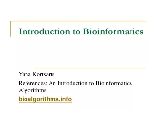
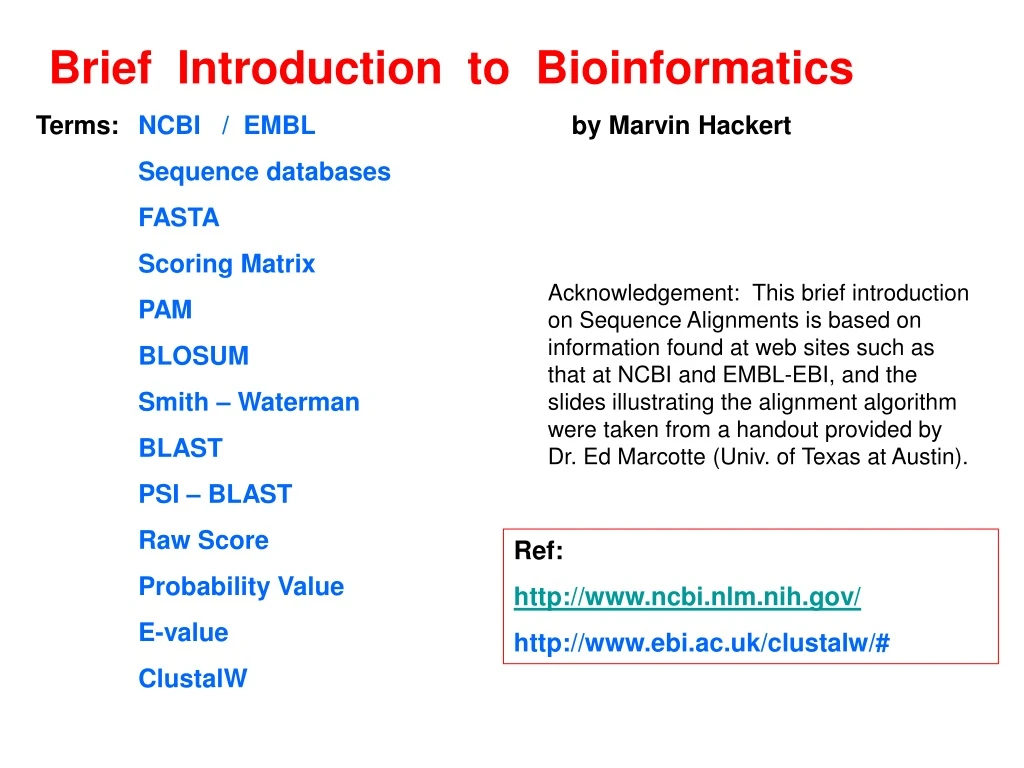
1. Brief Introduction to Bioinformatics Terms: NCBI / EMBL by Marvin Hackert Sequence databases FASTA Scoring Matrix PAM BLOSUM Smith – Waterman BLAST PSI – BLAST Raw Score Probability Value E-value ClustalW Acknowledgement: This brief introduction on Sequence Alignments is based on information found at web sites such as that at NCBI and EMBL-EBI, and the slides illustrating the alignment algorithm were taken from a handout provided by Dr. Ed Marcotte (Univ. of Texas at Austin). Ref: http://www.ncbi.nlm.nih.gov/ http://www.ebi.ac.uk/clustalw/#

4. Computational biology & Bioinformatics Computational biology and bioinformatics focus on the computational/ theoretical study of biological processes, and much of the disciplines involve constructing models like those above, then testing/validating/proving/applying these models using computers, hence the nickname “in silico biology”. The fields are closely related: computational biology is the more inclusive name, and bioinformatics often refers more specifically to the use of “informatics” tools like databases and data mining. Big problems tackled by these fields include: Assembling complete genomes from pieces of sequenced DNA Finding genes in genomes Modeling networks & interactions of proteins Predicting protein/RNA folding, structure, and function Sequence alignments

5. Sequence Alignment Let us look at a simple model for protein sequence evolution, and see how that allows us to align amino acid sequences of proteins to see if the proteins are related. This is the Smith-Waterman algorithm. The popular program BLAST is designed to mimic this algorithm, but BLAST is much faster due to some shortcuts and approximations and clever programming tricks. In general, biology can be thought of as the study of variations on a theme. Every modern organism inherited its traits, with minor random changes, from its parents. At the molecular level, this corresponds to sequences of DNA, RNA, and proteins that are very similar, but not identical, between the parents and progeny. This process of gene evolution can be modeled as a stochastic process of gene mutation followed by a “selection” process for those sequences still capable of performing their given roles in the cell. Over enough time, as new species evolve & diverge from related species, this has the result of producing families of related gene sequences, more similar in regions where that particular sequence is critical for the function of the molecule, and less similar in regions less critical for the molecule’s function. Frequently, we observe only the products of millions of years of this process. Given a set of molecules (DNA, RNA or protein sequences) - ?? How can we decide if they are similar enough to be considered part of the same family or if the observed similarity is just present by random chance.

6. Database Searching The Assumptions: The sequences being sought have an evolutionary ancestral sequence in common with the query sequence (our newly determined sequence). Our best guess at the actual path of evolution is the path that requires the fewest evolutionary events. All substitutions are not equally likely and should be weighted to account for this. Gaps: Insertions and deletions are less likely than substitutions and should be weighted to account for this.In most alignment and search programs, the gap penalty consists of two terms, the cost to open the gap and the cost to extend the gap.

7. Homology “Homology” is a much-misused term. Homology existed in biology long before the notion of protein sequences. It is not correct to state that two proteins are "30% homologous" with each other. Homology, relatednessor similarity attributed to descent from a common evolutionary ancestor, is not directly observable. What we observe in sequence database searching is sequence likeness or similarity. If the similarity is great enough we are allowed to make the scientific inference that the two sequences are homologous. Much of the previously determined knowledge we apply in database searching involves how to best measure sequence likeness, and how to determine whether the observed degree of sequence similarity or likeness is sufficient to allow us to infer that the sequences are homologous.

8. FASTAFormat

9. Examples of aligned protein sequences: Shown are 3 pairs of sequences, showing aligned sequences of proteins named FlgA1, FlgA2, FlgA3, and HvcPP. Between each pair the perfect matches and close matches (shown by + symbols, indicating chemically similar amino acids) are written. Two biologically related proteins with similar sequences: FlgA1 EAGNVKLKRGRLDTLPPRTVLDINQLVDAISLRDLSPDQPIQLTQFRQAWRVKAGQRVNVIASGD ++K+K+GRLDTLPP +L+ N A+SLR ++ QP+ R+ W +KAGQ V V+A G+ FlgA2 TLQDIKMKQGRLDTLPPGALLEPNFAQGAVSLRQINAGQPLTRNMLRRLWIIKAGQDVQVLALGE (186) Also biologically related (& fold up into the same 3D protein structure): FlgA1 EAGNVKLKRGRLDTLPPRTVLDINQLVDAISLRDLSPDQPIQLTQFRQAWRVKAGQRVNVIASGD A + P +L I+ R L P + I R+AW V+ G V V FlgA3 LAALKQVTLIAGKHKPDAMATHAEELQGKIAKRTLLPGRYIPTAAIREAWLVEQGAAVQVFFIAG (50) But these are biologically unrelated (& fold up into unrelated structures): FlgA1 AGNVKLKRGRLDTLPPRTVLDINQLVDAISLRDLSPDQPIQLTQFRQA-WRVKAGQRVNVIASGD AG+V K G + + PRT ++ I+ P PI +++A WRV A + V V+ GD HvcPP AGHV--KNGTMRIVGPRTCSNVWNGTFPINATTTGPSIPIPAPNYKKALWRVSATEYVEVVRVGD(128) The problem we face is how to distinguish the biologically meaningless match (FlgA1-HvcPP) from the biologically meaningful ones (FlgA1-FlgA2 and FlgA1-FlgA3)?

10. To align two sequences, we need: 1. Some way to decide which alignments are better than others. For this, we’ll invent a way to give the alignments a “score” indicating their quality. “Scoring Matrix” 2. Some way to align the proteins so that they get the best possible score. Smith-Waterman algorithm dynamic programming, recursive manner 3. Then finally, some way to decide when a score is “good enough” for us to believe the alignment is biologically significant. “Scramblings - Expect Values” extreme value distribution

11. What is a scoring matrix? The aim of a sequence alignment, is to match "the most similar elements" of two sequences. This similarity must be evaluated somehow. For example, consider the following two alignments: AIWQH AIWQH AL--QH A--LQH They seem quite similar: both contain one “gap" and one “substitution,” just at different positions. However, the first alignment is the better one because isoleucine (I) and leucine (L) are similar sidechains, while tryptophan (W) has a very different structure. This is a physico-chemical measure; we might prefer these days to say that leucine simply substitutes for isoleucine more frequently---without giving an underlying "reason" for this observation. However we explain it, it is much more likely that a mutation changed I into L and that W was lost, than W was changed into L and I was lost. We would expect that a change from I to L would not affect the function as much as a mutation from W to L---but this deserves its own topic. To quantify the similarity achieved by an alignment, scoring matrices are used: they contain a value for each possible substitution, and the alignment score is the sum of the matrix's entries for each aligned amino acid pair. For gaps a special gap score is necessary---just add a constant penalty score for each new gap. The optimal alignment is the one which maximizes the alignment score.

12. Importance of scoring matrices Scoring matrices appear in all analysis involving sequence comparison. The choice of matrix can strongly influence the outcome of the analysis. Scoring matrices implicitly represent a particular theory of evolution. Understanding theories underlying a given scoring matrix can aid in making proper choice. Types of matrices PAMBLOSSUMGONNETDNA Identity Matrix Ref: http://www.ebi.ac.uk/clustalw/#

13. Unitary Scoring Matrices Early sequence alignment programs used unitary scoring matrix. A unitary matrix scores all matches the same and penalizes all mismatches the same. Although this scoring is sometimes appropriate for DNA and RNA comparisons, for protein alignments using a unitary matrix amounts to proclaiming ignorance about protein evolution and structure. Thirty years of research in aligning protein sequences have shown that different matches and mismatches among the 400 amino acid pairs that are found in alignments require different scores. Many alternatives to the unitary scoring matrix have been suggested. One of the earliest suggestions was scoring matrix based on the minimum minimum number of bases that must be changed to convert a codon for one amino acid into a codon for a second amino acid. This matrix, known as the minimum mutation distance matrix, has succeeded in identifying more distant relationships among protein sequences than the unitary matrix approach.

14. Evolutionary Distances and log-odds scores The best improvement achieved over the unitary matrix was based on evolutionary distances. Margaret Dayhoff pioneered this approach in the 1970's. She made an extensive study of the frequencies in which amino acids substituted for each other during evolution. The studies involved carefully aligning all of the proteins in several families of proteins and then constructing phylogenetic trees for each family. Each phylogenetic tree was examined for the substitutions found on each branch. This lead to a table of the relative frequencies with which amino acids replace each other over a short evolutionary period. This table and the relative frequency of occurrence of the amino acids in the proteins studied were combined in computing the PAM (Point Accepted Mutations) family of scoring matrices. From a biological point of view PAM matrices are based on observed mutations. Thus they contain information about the processes that generate mutations as well as the criteria that are important in selection and in fixing a mutation within a population. From a statistical point of view PAM matrices, and other log-odds matrices, are the most accurate description of the changes in amino acid composition that are expected after a given number of mutations that can be derived from the data used in creating the matrices. Thus the highest scoring alignment is the statistically most likely to have been generated by evolution rather than by chance.

15. Log-odds matrices: Each score in the matrix is the logarithm of an odds ratio. The odds ratio used is the ratio of the number of times residue "A" is observed to replace residue "B" divided by the number of times residue "A" would be expected to replace residue "B" if replacements occurred at random. Thus positive scores in the matrix designate a pair of residues that replace each other more often than expected by chance. This is evidence in favor of the aligned sequences being homologous (that is, related to each other by through common ancestral gene). Negative scores in the matrix designate pairs of residues that replace each other less often than would be expected by chance and are evidence against the sequences being homologous. The BLOSUM family of matrices developed by Steven and Jorja Henikoff are one of these newly developed log-odds scoring matrices. The wide spread practical use and of systematic comparisons of the effectiveness of these matrices suggest that the BLOSUM matrices are an improvement over the Dayhoff PAM matrices. The improved performance of the BLOSUM matrices probably derives from two main factors. First is that many more protein sequences were known when the BLOSUM matrices were first derived and thus they incorporate many more observed amino acid substitutions. The second factor is that the observed substitutions used in constructing the BLOSUM matrices are restricted to those substitutions found within well conserved blocks in a multiple sequence alignment.

16. PAM (Percent Accepted Mutation) A unit introduced by M.O. Dayhoff et al. to quantify the amount of evolutionary change in a protein sequence. 1.0 PAM unit, is the amount of evolution which will change, on average, 1% of amino acids in a protein sequence. A PAM(x) substitution matrix is a look-up table in which scores for each amino acid substitution have been calculated based on the frequency of that substitution in closely related proteins that have experienced a certain amount (x) of evolutionary divergence. PAM matrices are based on global alignments of closely related proteins. The PAM1 is the matrix calculated from comparisons of sequences with no more than 1% divergence. Other PAM matrices are extrapolated from PAM1. Thus, using the PAM 250 scoring matrix means that about 250 mutations per 100 amino acids may have happened, while with PAM 10 only 10 mutations per 100 amino acids are assumed, so that only very similar sequences will reach useful alignment scores. The optimal alignment of two very similar sequences with PAM 500 may be less useful than that with PAM 50.

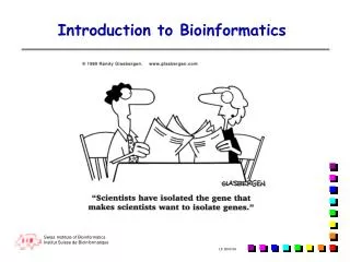
17. The colored regions in the figure above mark one possible grouping of such positive scores. These regions provide an objective basis for defining conservative substitutions, namely as amino acids that replace each other more frequently than would be expected from random replacements.

18. BLOSUM matrices are based on local alignments. BLOSUM (BLOcks SUbstitution Matrix): BLOSUM 62 is a matrix calculated from comparisons of sequences with no less than 62% divergence. BLOSUM 62 is the default matrix in BLAST 2.0. Though it is tailored for comparisons of moderately distant proteins, it performs well in detecting closer relationships. A search for distant relatives may be more sensitive with a different matrix. Differences between PAM and BLOSUM PAM matrices are based on an explicit evolutionary model (that is, replacements are counted on the branches of a phylogenetic tree), whereas the BLOSUM matrices are based on an implicit rather than explicit model of evolution. The sequence variability in the alignments used to count replacements. The PAM matrices are based on mutations observed throughout a global alignment, this includes both highly conserved and highly mutable regions. The BLOSUM matrices are based only on highly conserved regions in series of alignments forbidden to contain gaps.

19. BLOSUM62 Substitution Scoring Matrix. The BLOSUM 62 matrix is a 20 x 20 matrix in which every possible identity and substitution is assigned a score based on the observed frequencies of such occurences in alignments of related proteins.Identities are assigned the most positive scores.Frequently observed substitutions also receive positive scores and seldom observed substitutions are given negative scores.

21. Sequnce Analysis: Which scoring method should I use? The entropy as defined by information theory is the average amount of information per position in a sequence alignment that is available to determine whether or not the sequences are homologous. This amount of entropy is available only if the similarity scores used in the database search or alignment are matched for the appropriate degree of sequence divergence.

22. An Alignment Algorithm If we had all the time in the world, we could just make all possible alignments, score them all, & choose the best. But realistically, that won’t work, since even for two 100 amino acid sequences, there are 1059 possible alignments. So, the following approach was developed. The particular class of algorithm we’ll use is called dynamic programming, which refers to a set of algorithms that allow the optimal solutions to be found for problems that can be defined in a recursive manner. That is, the problems are broken into subproblems, which are in turn broken into subproblems, etc, until the simplest subproblems can be solved. For sequence alignments, this sequential dependency takes a form where the choice of optimal alignment of a sequence of length n is found from the solution to the optimal alignment of a sequence of length n-1 plus the alignment of the nth symbol, and the optimal alignment of the n-1 case is a function of the n-2 case, and so on. Dynamic programming was developed by Richard Bellman 40-50 years ago, but then “rediscovered” by biologists aligning sequences in the 1970’s.

23. There are 2 types of alignments that we could make: globaland local Global alignments will require a forced match between every symbol of one string with some symbol (or gap) of the second string, e.g. ACGTTATGCATGACGTA -C---ATGCAT----T- Local alignments will correspond to the best matching subsequences (including gaps). For the above example, this corresponds to: ATGCAT ATGCAT We’ll look at local alignments, since these are what are used in almost any sequence alignment algorithm you might choose. This approach (in biology) is named the Smith-Waterman algorithm after Temple Smith & Mike Waterman, Journal of Molecular Biology vol. 147, 195-197 (1981).

24. 1) H E A G A W G H E E 2) P A W H E A E

25. 1) H E A G A W G H E E 2) A W - H E

26. GAPS / Gap peanaties In most alignment and search programs, the gap penalty consists of two terms, thecost to open the gapand thecost to extend the gap. Ref: http://www.ebi.ac.uk/clustalw/#

27. Examples of aligned protein sequences: Shown are 3 pairs of sequences, showing aligned sequences of proteins named FlgA1, FlgA2, FlgA3, and HvcPP. Between each pair the perfect matches and close matches (shown by + symbols, indicating chemically similar amino acids) are written. Two biologically related proteins with similar sequences: FlgA1 EAGNVKLKRGRLDTLPPRTVLDINQLVDAISLRDLSPDQPIQLTQFRQAWRVKAGQRVNVIASGD ++K+K+GRLDTLPP +L+ N A+SLR ++ QP+ R+ W +KAGQ V V+A G+ FlgA2 TLQDIKMKQGRLDTLPPGALLEPNFAQGAVSLRQINAGQPLTRNMLRRLWIIKAGQDVQVLALGE (186) Also biologically related (& fold up into the same 3D protein structure): FlgA1 EAGNVKLKRGRLDTLPPRTVLDINQLVDAISLRDLSPDQPIQLTQFRQAWRVKAGQRVNVIASGD A + P +L I+ R L P + I R+AW V+ G V V FlgA3 LAALKQVTLIAGKHKPDAMATHAEELQGKIAKRTLLPGRYIPTAAIREAWLVEQGAAVQVFFIAG (50) But these are biologically unrelated (& fold up into unrelated structures): FlgA1 AGNVKLKRGRLDTLPPRTVLDINQLVDAISLRDLSPDQPIQLTQFRQA-WRVKAGQRVNVIASGD AG+V K G + + PRT ++ I+ P PI +++A WRV A + V V+ GD HvcPP AGHV--KNGTMRIVGPRTCSNVWNGTFPINATTTGPSIPIPAPNYKKALWRVSATEYVEVVRVGD(128) The problem we face is how to distinguish the biologically meaningless match (FlgA1-HvcPP) from the biologically meaningful ones (FlgA1-FlgA2 and FlgA1-FlgA3)?

28. 1) H E A G A W G H E E 2) A W - H E How do we know when a score is “good enough”? Two elements of aligning sequences: scoring the alignments (by generating substitution matrices) constructing the optimal scoring alignments by dynamic programming. After we get an alignment, we have to decide if score is “good enough” to be significant. One way to this is to ask how hard it is to get that score from random alignments. Suppose we “scrambled” one of the sequences, and found the best alignment with the other sequence. The algorithm will always give us an alignment, even though the score is not very good. Still, let’s do the scrambling and alignment process 1000 times. If we look at those scores, and never see a score as good as the real one, we can say that the real one has a 1 in a 1000 chance of happening just by luck. If we did this 1,000,000 times and still didn’t see a score that good, we would begin to feel pretty confident in our alignment being significant.

29. If we want, we could just do these million random tests after an alignment, & that would give us a perfectly correct feeling for how good the alignment was. However, in practice, we can get away with just doing a few random trials, then mathematically modeling the scores we get out to save having to do a million such trials. This is what is actually done.  The histogram of scores turns out to have a particular, predictable shape known as the extreme value distribution (also called the Gumbel distribution). Visually, the extreme value distribution looks this: This distribution can be described by an equation of the form: where N is the number of scrambled y's we tested, m is the mean value of the high scores from the scrambling experiment, and k and l are numbers that characterize the shape of the particular extreme value distribution that comes from aligning x to y. In practice, we can fit k and l from the scores we get from a few random alignments, we do a few scramblings, find k and l, then calculate the probability of seeing the real alignment score by chance from the equation above. If this is very low, say less than one in a thousand, we might begin to believe the two proteins are actually related.

30. Steps in doing a Multiple Sequence Alignment: • Get desired sequence in FASTA format. • NCBI web site – BLAST run • Select best matches to use in alignment • EMBL web site – ClustalW run >CgX SEQUENCE MPTYTCWSQRIRISREAKQRIAEAITDAHHELAHAPKYLVQVIFNEVEPDSYFIAAQSASENHIWVQATIRSGRTEKQKEELLLRLTQEIALILGIPNEEVWVYITEIPGSNMTEYGRLLMEPGEEEKWFNSLPEGLRERLTELEGSSE

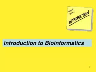
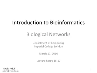
31. 4-OT– (Tautomerase/MIF Superfamily) - with Professor Chris Whitman (Pharmacy) Christian P. Whitman EEEEEEETT HHHHHHHHHHHHHHHHHHHT GGG EEEEEEE GGG EETTEETTTT 4OT 1 PIAQIHILEG_RSDEQKETLIREVSEAISRSLDAPLTSVRVIITEMAKGHFGIGGELASKVRR 62 CHMI 1 PHFIVECSDNIREEADLPGLFAKVNPTLAATGIFPLAGIRSRVHWVDTWQMADGQHDYAFVHM..-125 MIF 1 PMFIVNTNVP_RASVPEGFLSELTQQLAQATGK_PAQYIAVHVVPDQLMTFSGTNDPCALCSL..-114 A) B) C) Ref: Taylor, A.B., Czerwinski, R.M., Johnson, W.H., Whitman, C.P., and Hackert, M.L., "Crystal Structure of 4-Oxalocrotonate Tautomerase Inactivated by 2-Oxo-3-pentynotate at 2.4Å resolution: Analysis and Implications for the Mechanism of Inactivation and Catalysis" Biochemistry,37, 14692-14700 (1998).

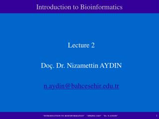
32. 4-OT - Tautomerase 4OT Homologues CHMI - Isomerase MIF - Cytokine / Hormone Dehalogenase Decarboxylase a a a (ab) 6 3 2 3

33. Sample Psi-BLAST Output Jinghui Zhang, Zheng Zhang, Webb Miller, and David J. Lipman (1997), "Gapped BLAST and PSI-BLAST: a new generation of protein database searchprograms", Nucleic Acids Res. 25:3389-3402. RID: 1012187428-16844-19639 Query= Pseudomonas putida - 4-OT (62 letters) 1 piaqihileg rsdeqketli revseaisrs ldapltsvrv iitemakghf giggelaskv rr Database: All non-redundant GenBank CDS translations+PDB+SwissProt+PIR+PRF 857,413 sequences; 270,034,499 total letters ********************* Sequences with E-value BETTER than threshold Round 1 – 30 Hits / Round 2 57 hits / Round 3 - 66 Hits Sequences with E-value BETTER than threshold Score E Sequences producing significant alignments: (bits) Valuegi|6624277|dbj|BAA88507.1| (AB029044) 4-oxalocrotonate isomerase... 81 2e-15 gi|16124116|ref|NP_407429.1| (NC_003143) putative tautomerase [Y... 78 2e-14 gi|14715457|dbj|BAB62059.1| (D85415) 4-oxalocrotonate tautomeras... 78 2e-14 gi|15642664|ref|NP_232297.1| (NC_002505) 5-carboxymethyl-2-hydro... 44 3e-04 gi|15801678|ref|NP_287696.1| (NC_002655) ydcE gene product [Esch... 44 3e-04 gi|16079011|ref|NP_389834.1| (NC_000964) similar to hypothetical... 43 8e-04 ******************* Sequences with E-value WORSE than threshold gi|15894207|ref|NP_347556.1| (NC_003030) Protein related to MIFH... 38 0.014 gi|14600626|ref|NP_147143.1| (NC_000854) MRSA protein [Aeropyrum... 37 0.047 gi|17562710|ref|NP_506003.1| (NM_073602) macrophage migration in... 35 0.16 gi|5051891|gb|AAD38354.1| (AF119571) macrophage migration inhibi... 30 4.4 gi|14600626|ref|NP_147143.1| (NC_000854) MRSA protein [Aeropyrum... 30 4.6 gi|5327268|emb|CAB46354.1| (AJ012740) macrophage migration inhib... 30 8.1