Download
1 / 48
500 likes | 642 Vues
Extrapolation: Reaching Beyond the Data. Linear models give a predicted value for each case in the data. We cannot assume that a linear relationship in the data exists beyond the range of the data.

E N D
Extrapolation: Reaching Beyond the Data • Linear models give a predicted value for each case in the data. • We cannot assume that a linear relationship in the data exists beyond the range of the data. • The farther the new x value is from the mean in x, the less trust we should place in the predicted value. • Once we venture into new x territory, such a prediction is called an extrapolation.
Extrapolation (cont.) • Extrapolations are dubious because they require the additional—and very questionable — assumption that nothing about the relationship between x and y changes even at extreme values of x. • Extrapolations can get you into deep trouble. You’re better off not making extrapolations.
Extrapolation (cont.) • Here is a timeplot of the Energy Information Administration (EIA) predictions and actual prices of oil barrel prices. How did forecasters do? • They seemed to have missed a sharp run-up in oil prices in the past few years.
Predicting the Future • Extrapolation is always dangerous. But, when the x-variable in the model is time, extrapolation becomes an attempt to peer into the future. • Knowing that extrapolation is dangerous doesn’t stop people. The temptation to see into the future is hard to resist. • Here’s some more realistic advice: If you must extrapolate into the future, at least don’t believe that the prediction will come true.
Outliers, Leverage, and Influence • Outlying points can strongly influence a regression. Even a single point far from the body of the data can dominate the analysis. • Any point that stands away from the others can be called an outlier and deserves your special attention.
Outliers, Leverage, and Influence • Outlying points can strongly influence a regression. Even a single point far from the body of the data can dominate the analysis. • Any point that stands away from the others can be called an outlier and deserves your special attention.
Outliers, Leverage, and Influence (cont.) • The following scatterplot shows that something was awry in Palm Beach County, Florida, during the 2000 presidential election…
Outliers, Leverage, and Influence (cont.) • The red line shows the effects that one unusual point can have on a regression:
Outliers, Leverage, and Influence (cont.) • A data point can also be unusual if its x-value is far from the mean of the x-values. Such points are said to have high leverage.
Outliers, Leverage, and Influence (cont.) • A point with high leverage has the potential to change the regression line. • We say that a point is influential if omitting it from the analysis gives a very different model.
Outliers, Leverage, and Influence (cont.) • The extraordinarily large shoe size gives the data point high leverage. Wherever the IQ is, the line will follow!
Outliers, Leverage, and Influence (cont.) • When we investigate an unusual point, we often learn more about the situation than we could have learned from the model alone. • You cannot simply delete unusual points from the data. You can, however, fit a model with and without these points as long as you examine and discuss the two regression models to understand how they differ.
Outliers, Leverage, and Influence (cont.) • Warning: • Influential points can hide in plots of residuals. • Points with high leverage pull the line close to them, so they often have small residuals. • You’ll see influential points more easily in scatterplots of the original data or by finding a regression model with and without the points.
Lurking Variables and Causation • No matter how strong the association, no matter how large the R2value, no matter how straight the line, there is no way to conclude from a regression alone that one variable causes the other. • There’s always the possibility that some third variable is driving both of the variables you have observed. • With observational data, as opposed to data from a designed experiment, there is no way to be sure that a lurking variable is not the cause of any apparent association.
Lurking Variables and Causation (cont.) • The following scatterplot shows that the average life expectancy for a country is related to the number of doctors per person in that country:
Lurking Variables and Causation (cont.) • This new scatterplot shows that the average life expectancy for a country is related to the number of televisions per person in that country:
Straight to the Point • We cannot use a linear model unless the relationship between the two variables is linear. Often re-expression can save the day, straightening bent relationships so that we can fit and use a simple linear model. • Two simple ways to re-express data are with logarithms and reciprocals. • Re-expressions can be seen in everyday life—everybody does it.
Straight to the Point (cont.) • The relationship between fuel efficiency (in miles per gallon) and weight (in pounds) for late model cars looks fairly linear at first:
Straight to the Point (cont.) • A look at the residuals plot shows a problem:
Straight to the Point (cont.) • We can re-express fuel efficiency as gallons per hundred miles (a reciprocal) and eliminate the bend in the original scatterplot:
Straight to the Point (cont.) • A look at the residuals plot for the new model seems more reasonable:
Goals of Re-expression • Goal 1: Make the distribution of a variable (as seen in its histogram, for example) more symmetric.
Goals of Re-expression (cont.) • Goal 2: Make the spread of several groups (as seen in side-by-side boxplots) more alike, even if their centers differ.
Goals of Re-expression (cont.) • Goal 3: Make the form of a scatterplot more nearly linear.
Goals of Re-expression (cont.) • Goal 4: Make the scatter in a scatterplot spread out evenly rather than thickening at one end. • This can be seen in the two scatterplots we just saw with Goal 3:
The Ladder of Powers • There is a family of simple re-expressions that move data toward our goals in a consistent way. This collection of re-expressions is called the Ladder of Powers. • The Ladder of Powers orders the effects that the re-expressions have on data.
Power Name Comment 2 Square of data values Try with unimodal distributions that are skewed to the left. 1 Raw data Data with positive and negative values and no bounds are less likely to benefit from re-expression. ½ Square root of data values Counts often benefit from a square root re-expression. “0” We’ll use logarithms here Measurements that cannot be negative often benefit from a log re-expression. –1/2 Reciprocal square root An uncommon re-expression, but sometimes useful. –1 The reciprocal of the data Ratios of two quantities (e.g., mph) often benefit from a reciprocal. The Ladder of Powers
Fat Versus Protein: An Example • The following is a scatterplot of total fat versus protein for 30 items on the Burger King menu:
A negative residual means the predicted value’s too big (an overestimate). A positive residual means the predicted value’s too small (an underestimate). In the figure, the estimated fat of the BK Broiler chicken sandwich is 36 g, while the true value of fat is 25 g, so the residual is –11 g of fat. Residuals (cont.)
Residuals Revisited • The linear model assumes that the relationship between the two variables is a perfect straight line. The residuals are the part of the data that hasn’t been modeled. Data = Model + Residual or (equivalently) Residual = Data – Model Or, in symbols,
Residuals Revisited (cont.) • Residuals help us to see whether the model makes sense. • When a regression model is appropriate, nothing interesting should be left behind. • After we fit a regression model, we usually plot the residuals in the hope of finding…nothing.
The Residual Standard Deviation • The standard deviation of the residuals, se, measures how much the points spread around the regression line. • Check to make sure the residual plot has about the same amount of scatter throughout. Check the Equal Variance Assumption with the Does the Plot Thicken? Condition. • We estimate the SD of the residuals using:
The Residual Standard Deviation • We don’t need to subtract the mean because the mean of the residuals • Make a histogram or normal probability plot of the residuals. It should look unimodal and roughly symmetric. • Then we can apply the 68-95-99.7 Rule to see how well the regression model describes the data.
R2—The Variation Accounted For • The variation in the residuals is the key to assessing how well the model fits. • In the BK menu items example, total fat has a standard deviation of 16.4 grams. The standard deviation of the residuals is 9.2 grams.
R2—The Variation Accounted For (cont.) • If the correlation were 1.0 and the model predicted the fat values perfectly, the residuals would all be zero and have no variation. • As it is, the correlation is 0.83—not perfection. • However, we did see that the model residuals had less variation than total fat alone. • We can determine how much of the variation is accounted for by the model and how much is left in the residuals.
R2—The Variation Accounted For (cont.) • The squared correlation, r2, gives the fraction of the data’s variance accounted for by the model. • Thus, 1 – r2 is the fraction of the original variance left in the residuals. • For the BK model, r2 = 0.832= 0.69, so 31% of the variability in total fat has been left in the residuals.
R2—The Variation Accounted For (cont.) • All regression analyses include this statistic, although by tradition, it is written R2(pronounced “R-squared”). An R2of 0 means that none of the variance in the data is in the model; all of it is still in the residuals. • When interpreting a regression model you need to Tell what R2means. • In the BK example, 69% of the variation in total fat is accounted for by variation in the protein content.
How Big Should R2 Be? • R2is always between 0% and 100%. What makes a “good” R2value depends on the kind of data you are analyzing and on what you want to do with it. • The standard deviation of the residuals can give us more information about the usefulness of the regression by telling us how much scatter there is around the line.
Reporting R2 • Along with the slope and intercept for a regression, you should always report R2so that readers can judge for themselves how successful the regression is at fitting the data. • Statistics is about variation, and R2measures the success of the regression model in terms of the fraction of the variation of y accounted for by the regression.
Assumptions and Conditions • Quantitative Variables Condition: • Regression can only be done on two quantitative variables (and not two categorical variables), so make sure to check this condition. • Straight Enough Condition: • The linear model assumes that the relationship between the variables is linear. • A scatterplot will let you check that the assumption is reasonable.
Assumptions and Conditions (cont.) • If the scatterplot is not straight enough, stop here. • You can’t use a linear model for any two variables, even if they are related. • They must have a linear association or the model won’t mean a thing. • Some nonlinear relationships can be saved by re-expressing the data to make the scatterplot more linear.
Assumptions and Conditions (cont.) • It’s a good idea to check linearity again after computing the regression when we can examine the residuals. • Does the Plot Thicken? Condition: • Look at the residual plot -- for the standard deviation of the residuals to summarize the scatter, the residuals should share the same spread. Check for changing spread in the residual scatterplot.
Assumptions and Conditions (cont.) • Outlier Condition: • Watch out for outliers. • Outlying points can dramatically change a regression model. • Outliers can even change the sign of the slope, misleading us about the underlying relationship between the variables. • If the data seem to clump or cluster in the scatterplot, that could be a sign of trouble worth looking into further.
Reality Check: Is the Regression Reasonable? • Statistics don’t come out of nowhere. They are based on data. • The results of a statistical analysis should reinforce your common sense, not fly in its face. • If the results are surprising, then either you’ve learned something new about the world or your analysis is wrong. • When you perform a regression, think about the coefficients and ask yourself whether they make sense.
What Can Go Wrong? • Don’t fit a straight line to a nonlinear relationship. • Beware extraordinary points (y-values that stand off from the linear pattern or extreme x-values). • Don’t extrapolate beyond the data—the linear model may no longer hold outside of the range of the data. • Don’t infer that x causes y just because there is a good linear model for their relationship—association is not causation. • Don’t choose a model based on R2alone.
What have we learned? (cont.) • The correlation tells us several things about the regression: • The slope of the line is based on the correlation, adjusted for the units of x and y. • For each SD in x that we are away from the x mean, we expect to be r SDs in y away from the y mean. • Since r is always between –1 and +1, each predicted y is fewer SDs away from its mean than the corresponding x was (regression to the mean). • R2 gives us the fraction of the response accounted for by the regression model.
What have we learned? • The residuals also reveal how well the model works. • If a plot of the residuals against predicted values shows a pattern, we should re-examine the data to see why. • The standard deviation of the residuals quantifies the amount of scatter around the line.
What have we learned? (cont.) • The linear model makes no sense unless the Linear Relationship Assumption is satisfied. • Also, we need to check the Straight Enough Condition and Outlier Condition with a scatterplot. • For the standard deviation of the residuals, we must make the Equal Variance Assumption. We check it by looking at both the original scatterplot and the residual plot for Does the Plot Thicken? Condition.