Download
1 / 35
360 likes | 828 Vues
Chapter 7: Normal Probability Distributions. In Chapter 7:. 7.1 Normal Distributions 7.2 Determining Normal Probabilities 7.3 Finding Values That Correspond to Normal Probabilities 7.4 Assessing Departures from Normality. § 7.1: Normal Distributions.

E N D
Chapter 7: Normal Probability Distributions 7: Normal Probability Distributions
In Chapter 7: 7.1 Normal Distributions 7.2 Determining Normal Probabilities 7.3 Finding Values That Correspond to Normal Probabilities 7.4 Assessing Departures from Normality 7: Normal Probability Distributions
§7.1: Normal Distributions • This pdf is the most popular distribution for continuous random variables • First described de Moivre in 1733 • Elaborated in 1812 by Laplace • Describes some natural phenomena • More importantly, describes sampling characteristics of totals and means 7: Normal Probability Distributions
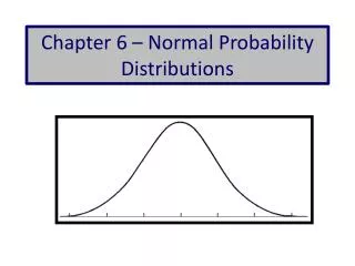
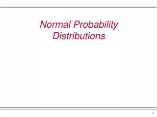
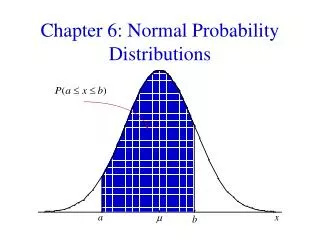
Figure: Age distribution of a pediatric population with overlying Normal pdf Normal Probability Density Function • Recall: continuous random variables are described with probability density function (pdfs) curves • Normal pdfs are recognized by their typical bell-shape 7: Normal Probability Distributions
Area Under the Curve • pdfs should be viewed almost like a histogram • Top Figure: The darker bars of the histogram correspond to ages ≤ 9 (~40% of distribution) • Bottom Figure: shaded area under the curve (AUC) corresponds to ages ≤ 9 (~40% of area) 7: Normal Probability Distributions
μ controls location σ controls spread Parameters μ and σ • Normal pdfs have two parameters μ- expected value (mean “mu”)σ- standard deviation (sigma) 7: Normal Probability Distributions
σ μ Mean and Standard Deviation of Normal Density 7: Normal Probability Distributions
Standard Deviation σ • Points of inflectionsone σbelow and above μ • Practice sketching Normal curves • Feel inflection points (where slopes change) • Label horizontal axis with σlandmarks 7: Normal Probability Distributions
Two types of means and standard deviations • The mean and standard deviation from the pdf (denoted μ and σ) are parameters • The mean and standard deviation from a sample (“xbar” and s) are statistics • Statistics and parameters are related, but are not the same thing! 7: Normal Probability Distributions
68-95-99.7 Rule forNormal Distributions • 68% of the AUC within ±1σ of μ • 95% of the AUC within ±2σ of μ • 99.7% of the AUC within ±3σ of μ 7: Normal Probability Distributions
Wechsler adult intelligence scores: Normally distributed with μ = 100 and σ = 15; X ~ N(100, 15) 68% of scores within μ ± σ= 100 ± 15 = 85 to 115 95% of scores within μ ± 2σ= 100 ± (2)(15) = 70 to 130 99.7% of scores in μ ± 3σ= 100 ± (3)(15) = 55 to 145 Example: 68-95-99.7 Rule 7: Normal Probability Distributions
… we can easily determine the AUC in tails 95% Symmetry in the Tails Because the Normal curve is symmetrical and the total AUC is exactly 1… 7: Normal Probability Distributions
Example: Male Height • Male height: Normal with μ= 70.0˝ and σ= 2.8˝ • 68% within μ ± σ = 70.0 2.8 = 67.2 to 72.8 • 32% in tails (below 67.2˝ and above 72.8˝) • 16% below 67.2˝ and 16% above 72.8˝ (symmetry) 7: Normal Probability Distributions
Reexpression of Non-Normal Random Variables • Many variables are notNormal but can be reexpressed with a mathematical transformationto be Normal • Example of mathematical transforms used for this purpose: • logarithmic • exponential • square roots • Review logarithmic transformations… 7: Normal Probability Distributions
Base 10 log function Logarithms • Logarithms are exponents of their base • Common log(base 10) • log(100) = 0 • log(101) = 1 • log(102) = 2 • Natural ln (base e) • ln(e0) = 0 • ln(e1) = 1 7: Normal Probability Distributions
Example: Logarithmic Reexpression Take exponents of “95% range” e−1.9,1.3 = 0.15 and 3.67 Thus, 2.5% of non-diseased population have values greater than 3.67 use 3.67 as screening cutoff • Prostate Specific Antigen (PSA) is used to screen for prostate cancer • In non-diseased populations, it is not Normally distributed, but its logarithm is: • ln(PSA) ~N(−0.3, 0.8) • 95% of ln(PSA) within= μ ± 2σ= −0.3± (2)(0.8) = −1.9 to 1.3 7: Normal Probability Distributions
§7.2: Determining Normal Probabilities When value do not fall directly on σ landmarks: 1. State the problem 2. Standardize the value(s) (z score) 3. Sketch, label, and shade the curve 4. Use Table B 7: Normal Probability Distributions
Step 1: State the Problem • What percentage of gestations are less than 40 weeks? • Let X ≡ gestational length • We know from prior research: X ~ N(39, 2) weeks • Pr(X ≤ 40) = ? 7: Normal Probability Distributions
Standard Normal variable≡ “Z” ≡ a Normal random variable with μ = 0 and σ = 1, Z ~ N(0,1) Use Table B to look up cumulative probabilities for Z Step 2: Standardize 7: Normal Probability Distributions
Example: A Z variable of 1.96 has cumulative probability 0.9750. 7: Normal Probability Distributions
Step 2 (cont.) Turn value into z score: z-score= no. of σ-units above (positive z) or below (negative z) distribution mean μ 7: Normal Probability Distributions
Steps 3 & 4: Sketch & Table B 3. Sketch 4. Use Table B to lookup Pr(Z ≤ 0.5) = 0.6915 7: Normal Probability Distributions
Probabilities Between Points a represents a lower boundary b represents an upper boundary Pr(a ≤ Z ≤ b) = Pr(Z ≤ b) − Pr(Z ≤ a) 7: Normal Probability Distributions
Between Two Points Pr(-2 ≤ Z ≤ 0.5) = Pr(Z ≤ 0.5) − Pr(Z ≤ -2).6687 = .6915 − .0228 .6687 .6915 .0228 -2 -2 0.5 0.5 See p. 144 in text 7: Normal Probability Distributions
§7.3 Values Corresponding to Normal Probabilities • State the problem • Find Z-score corresponding to percentile (Table B) • Sketch 4. Unstandardize: 7: Normal Probability Distributions
z percentiles • zp≡ the Normal z variable with cumulative probability p • Use Table B to look up the value of zp • Look inside the table for the closest cumulative probability entry • Trace the z score to row and column 7: Normal Probability Distributions
e.g., What is the 97.5th percentile on the Standard Normal curve? z.975 = 1.96 Notation: Let zp represents the z score with cumulative probability p, e.g., z.975= 1.96 7: Normal Probability Distributions
Step 1: State Problem Question: What gestational length is smaller than 97.5% of gestations? • Let X represent gestations length • We know from prior research that X ~ N(39, 2) • A value that is smaller than .975 of gestations has a cumulative probability of.025 7: Normal Probability Distributions
Step 2 (z percentile) Less than 97.5% (right tail) = greater than 2.5% (left tail) z lookup: z.025 = −1.96 7: Normal Probability Distributions
Unstandardize and sketch The 2.5th percentile is 35 weeks 7: Normal Probability Distributions
Same distribution on Normal “Q-Q” Plot 7.4 Assessing Departures from Normality Approximately Normal histogram Normal distributions adhere to diagonal line on Q-Q plot 7: Normal Probability Distributions
Negative Skew Negative skew shows upward curve on Q-Q plot 7: Normal Probability Distributions
Positive Skew Positive skew shows downward curve on Q-Q plot 7: Normal Probability Distributions
Same data as prior slide with logarithmic transformation The log transform Normalize the skew 7: Normal Probability Distributions
Leptokurtotic Leptokurtotic distribution show S-shape on Q-Q plot 7: Normal Probability Distributions