Download
1 / 53
530 likes | 648 Vues
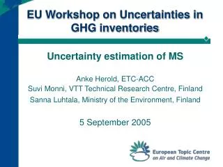
Methods to estimate uncertainties EU Workshop on uncertainties in greenhouse gas inventories. 5 to 6 th September 2005, Helsinki, Finland. John Watterson 1 , Justin Goodwin 1 , Melissa Downes 1 , Alistair Manning 2 , and Lorna Brown 3. With thanks to John Abbott 1 and Neil Passant 1.

E N D
Methods to estimate uncertaintiesEU Workshop on uncertainties in greenhouse gas inventories 5 to 6th September 2005, Helsinki, Finland. John Watterson1, Justin Goodwin1, Melissa Downes1,Alistair Manning2, andLorna Brown3 With thanks to John Abbott1 and Neil Passant1 1National Environmental Technology Centre - Netcen - Harwell Science Park, Didcot, Oxfordshire, OX11 0QJ, UK. 2The Met Office, FitzRoy Road, Exeter, Devon, EX1 3PB, UK. 3Institute of Grassland and Environmental Research (IGER), North Wyke Research Station, Okehampton, Devon, EX20 2SB, UK.
What is in this presentation Topics • Overview of methods and guidance – initial thoughts • Estimation of uncertainties in activity data (AD) • Use of IPCC default uncertainties in national inventories • Estimation of uncertainty in national emission factors (EFs) • Verification of emission data: How can comparison of different models/methods be used to estimate uncertainties? • Estimation of uncertainties in models • Combining uncertainties • Treatment of correlations
Some general problems with uncertainty analysis • Strictly uncertainties in inventories cannot be exactly quantified • Unknown sources • Gaps in understanding of existing sources • Measurement for emission factors are inadequate to quantify uncertainties • Emission factors may be inappropriate for specific sources • Expert elicitation has a role – workshops later this afternoon
However • We need to understand the likely magnitude of uncertainties and their impacts • But there is hope!! • We do have some knowledge and understanding of uncertainties • We need to identify major uncertainties to direct improvements in GHG inventories
Overview of methods and guidance • ‘Approach 1’ • emission sources aggregated up to level similar to IPCC Summary Table 7A • uncertainties then estimated for these categories • uncertainties calculated based on error propagation equations • Provides basis for Key Source analysis • ‘Approach 2’ • corresponds to Monte Carlo approach • Can use software such as @RISK and MS excel spreadsheets – or write your own MC code • Recommend reading the 2006 IPCC Guidelines – Volume 1 Chapter 3 “Uncertainties”
Estimation of uncertainties in activity data (AD) - examples Energy Digest of UK Energy Statistics(UK Department for Trade and Industry) Energy statistics for the UK (imports, exports, production, consumption, demand) of liquid, solid and gaseous fuels Calorific values of fuels and conversion factors Agriculture UK Defra - Institute of Grassland and Environmental Research (IGER)
Estimation of uncertainties in activity data (AD) Pollution Inventory(Environment Agency) Scottish Environmental Protection Agency United Kingdom Petroleum Industry Association United Kingdom Offshore Operators Association Iron and Steel Statistics Bureau Etc. Industrial Processes
Uncertainties in UK fuel activity data • Fuel activity data taken from Digest of UK Energy Statistics • Uncertainties used for the fuel activity data estimated from the statistical difference between supply and demand for each fuel • Effectively the residuals when a mass balance is performed on the production, imports, exports and consumption of fuels • For solid and liquid fuels both positive and negative results are obtained indicating that these are uncertainties rather than losses
Uncertainties in UK fuel activity data • Quoted uncertainty refers to the total fuel consumption rather than the consumption by a particular sector, e.g. residential coal • To avoid underestimating uncertainties, it was necessary to correlate the uncertainties used for the same fuel in different sectors
Uncertainties in UK fuel activity data • For gaseous fuels uncertainties include losses and tended to be negative. For natural gas, a correction was made to take account of leakage from the gas transmission system but for other gases this was not possible. • The uncertainties in activity data for minor fuels (colliery methane, orimulsion, SSF, petroleum coke) and non-fuels (limestone, dolomite and clinker) were estimated based on judgement comparing their relative uncertainty with that of the known fuels.
Difference in supply and demand of coal Trend suggests improvement in accuracy of estimates of supply and demand over time?
Difference in supply and demand of natural gas Supply greater than demand – is this all due to losses (fugitive emissions) in the gas transmission system? Could apply a correction if estimated fugitive emissions are known Decline in difference reflects measures implemented in the UK to reduce fugitive emissions in the gas transmission system
Some general comments on using statistical differences derived from energy balance data • Uncertainties in the fuel combustion data for specific sectors or applications, are probably higher than the uncertainty suggested by the statistical difference between supply and demand • Warning - if a statistical difference is zero it is likely that the data are of uncertain quality and this does not imply zero uncertainty. In these instances, the data quality should be examined for QA/QC purposes and the relevant statistical agencies should investigate
Using IPCC default uncertainties • Where possible, uncertainty data for EFs should be derived from published country specific studies • estimate values of uncertainties • you may be able to derive the PDF from available data • If such data are unavailable, then use default values from guidelines • suggest it will be best to refer to the 2006 IPCC guidelines which should be available in early 2006 • unless you have other evidence, assume PDF normal • before using defaults, try using expert judgement / elicitation to produce more applicable data
Typical data available in 2006 IPCC guidelines • Data above taken from Stationary Combustion Chapter in 2006 Guidelines • Derived from EMEP/CORINAIR Guidebook • Very limited sector specific information and wide range of uncertainty quoted • GLs suggest an overall uncertainty value of 7 % for the CO2 emission factors of Energy
Using uncertainties in the IPCC guidelines e.g. Uncertainties in CH4 emissions from Table 2.12 in previous slide Probability Distribution 50 150 100 = 1 standard deviation of the mean, E 2 = 50 95% CI = 2 / E = 50 / 100 = 50 %
Using uncertainties in the IPCC guidelines e.g. uncertainties in N2O emissions from Table 2.12 These are order of magnitude uncertainties – need to use Approach 2 (i.e. MC simulation) and define a suitable PDF
Estimation of uncertainty in national emission factors (EFs)
Example from data to support UK review of carbon emission factors (CEF) Large number of samples used to estimate CEF Checks to see if a weighted mean approach produces a more accurate CEF estimate
Verification of emission data: how can comparison of different models/methods be used to estimate uncertainties?
Initial considerations • One a very basic level comparisons using different models/methods can be used to assess uncertainties by • (a) The closeness of the estimates gives a feel for potential gross errors. It depends on how independent the methods are and the potential errors in each method ‑ both estimation and modeling approaches could have problems, but for different reasons. • (b) By comparison across a wide number of pollutants a qualitative feel for the uncertainty for any particular pollutant can be gauged.
Verification of the UK GHG inventory • The approach uses the Lagrangian dispersion model NAME (Numerical Atmospheric dispersion Modelling Environment) • Sorts the observations made at Mace Head into those that represent Northern Hemisphere baseline air masses and those that represent regionally-polluted air masses arriving from Europe. The Mace Head observations and the hourly air origin maps are applied in an inversion algorithm to estimate the magnitude and spatial distribution of the European emissions that best support the observations • The technique has been applied to 2-yearly rolling subsets of the data and used to estimate longer term averages
Verification of the UK GHG inventory • The inversion (best-fit) technique, simulated annealing, is used to fit the model emissions to the observations. • It assumes that the emissions from each grid box are uniform in both time and space over the duration of the data. This in turn implies that the release • is assumed independent of meteorological factors such as temperature and diurnal or annual cycles, and • that, in so far as the emission relates to industrial production or other anthropogenic activity, use there is no definite cycle or intermittency. • The estimated releases will include any natural release as well as anthropogenic emissions.
Based on meteorological analyses NAME model derived air origin maps Darker shade – Greater contribution from area All possible surface sources over previous 10 days Maps generated for each hour 1995-2004 Baseline analysis Mace Head
Inverse modelling • Aim: generate emission estimates from ‘polluted’ observations (above baseline) • Use NAME to predict concentration time series at Mace Head from each source • Scale emissions to obtain best match between model and observations • Simulated Annealing • Iterative technique • No prior information • Apply to all monitored species • Independent verification of emissions Equation: Ae = m Minimise: m - Ae A: the dilution matrix m: observed concentrations (- baseline) e: emissions
Nitrous oxide – comparison of GHG inventory estimates and model estimates Thermal oxidiser abatement system fitted to adipic acid plant
Quality of agreement between UK GHGI estimates and model • Reasonable agreement between modelled and measured which gives confidence of the inventory estimates • But fitment of abatement to adipic acid plant not reflected in NAME model trend • This problem investigated with representatives from the adipic acid plant and the meteorological office • Where was the problem – GHG inventory or model?
Answer – probably mostly the model, but check the GHG inventory also • The NAME model assumes no definite cycle or intermittency in emissions – this was not the case – periods were the adipic acid plant was shut down and periods where abatement not operating • So, make adjustments to the model • The oxidised nitrogen from wastewater is not currently included in the GHG – this (small) source could be added to improve the accuracy of the N2O estimate • So, make checks on the inventory
Initial considerations • Model is a representation of a ‘real world’ system – but can never exactly mimic the ‘real world’ • Key considerations in model uncertainty • Has the correct ‘real world’ been identified – for example, the ‘real world’ in a GHG inventory would be a complete and unbiased inventory • Is the model an accurate representation of this ‘real world’?
Example using N2O from agriculture in the UK GHG inventory Recent detailed study into the uncertainty of the model used to estimate emissions from the UK GHG inventory An inventory of nitrous oxide emissions from agriculture using the IPCC methodology: emission estimate, uncertainty and sensitivity analysis (2001). Brown, L., Amstrong Brown, S., Jarvis, S.C., Syed, B., Goulding, K.W.T., Philips, V.R., Sneath, R.W. and Pain, B.F. Atmos Environ., 35, 1439-1449.
Approach • Monte Carlo approach used to estimate the uncertainty in the model • 26 parameters were included • For some parameters, a beta pert distribution used derived from IPCC minima, maxima and most likely (default) values. No information in IPCC GLs to suggest alternative distribution. • Sensitivity analysis performed using multivariate stepwise regression using @RISK software
Results • N2O emissions from UK agriculture were estimated to be 87 Gg N2O-N for both 1990 and 1995 using the IPCC default EFs • Total estimate shown to have high overall uncertainty of 62% • Comparisons of results from this study and other UK-derived inventories suggests the default IPCC inventory may overestimate emissions • Uncertainty in individual components determined • This has identified the components of the model where improvements could be made since • emissions are a significant fraction of the total and • the associated uncertainties are high
Correlations When to use a correlation • Activity Data are calculated via mass balance • Supply and demand of fuels in energy statistics • Emission Factors are shared across activities • Natural gas or gas/diesel oil used by different sources • Emission Factors are calculated or extrapolated across a time series • Methane from livestock
Correlations (ii) How to use a correlation • Can be used in combination • Activity and EF’s correlated • If correlations occur, the easiest and most effective method is to use a Monte Carlo Simulation • NB: Correlations may not have an effect. Will only affect areas where the inventory is sensitive and/or the dependencies are very strong
Combining uncertainties • For Tier 2 analysis - a Monte Carlo approach is necessary. • Uncertainties are set and the correlations marked. The software is then set up and run and automatically takes these into account. • For component uncertainties <60%, a sum of squares approach can be used. • UT = (UE2 + UA2) • For component uncertainties >60% all that is possible is to combine limiting values to define an overall range • U% = (E+A+E*A/100) and L% = (E+A-E*A/100) • U=Uncertainty, T=total, E=Emission Factor, A=Activity Data, U%=upper limit, L%= lower limit
Calculating uncertainties Triangular Lognormal Uniform Fuel/Activity Uncertainty Emission Uncertainty Emission Factor Uncertainty Frequency Probability Distribution Value Min Max Range Distribution Types: normal
Tier 2 - Monte-Carlo Method Input 2 Model Result Input 1
Tier 2 - Monte-Carlo Method Factors Activity Min Min Min Min Max Max Max Max Emission • Step 1: Assess component uncertainties • Expert Judgement & Data • Maximum, Minimum • Distribution type • Step2: Run the analysis • up to 20,000 iterations • Step 3: Results • 5th - 95th percentile = Range as % of the mean Factors Activity Emission
Comments • Correlations do affect the overall uncertainty result – suggest approach is to start identifying inputs that are correlated, rather than setting up the model with the input level at the lowest level of aggregation and examining the correlations in each parameter individually • It is easy to produce MC output that superficially looks credible – but carefully check underlying assumptions • You can write a programme to complete a MC analysis – you do not need to use an expensive commercial package