Download
1 / 18
210 likes | 541 Vues
3. Laplace Transform. 3.1 Introduction. Laplace transform(L.T.) ; a mathematical tool that can significantly reduce the effort required to solve linear differential equation model.

E N D
3. Laplace Transform 3.1 Introduction • Laplace transform(L.T.) ; a mathematical tool that can significantly reduce the effort required to solve linear differential equation model. • Major benefit ; this transformation converts differential equations to algebraic equations, which can simplify the mathematical manipulations required to obtain a solution.
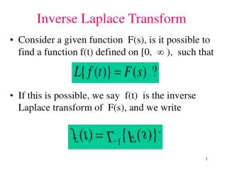
3.2 Laplace Transform of Representative Functions • Definition Where the function f(t) must satisfy conditions which include being piecewise continuous for . • Inverse transform ; • Property; Linear operator; it satisfies the general superposition principle.
Examples 1. Constant function , ( is a constant) 2. Unit step function
3. Derivatives • n-th order derivative where is the i-th derivative evaluated at t=0.
4. Exponential function if b<0, the real part of s must be restricted to be larger than -b for the integrated to be finite. 5. Trigonometric functions • Euler Identity
6. Rectangular pulse function Figure 3.1. The rectangular pulse function.
3.3 Solution of Differential Equations by Laplace Transform Techniques • Example; Solve the differential equation, using Laplace transform. Solution) Take Laplace transform both side of (3.19).
General solution procedure 1. Take the Laplace transform of both sides of the differential equation. 2. Solve for . • If the expression for dose not appear in table. • If the expression for not appear in table, go to Step 5. 3. Factor the characteristic equation polynomial. 4. Perform the Partial Fraction Expansion. 5. Use the inverse Laplace transform relations to find y(t).
3.4 Partial Fraction Expansion Example) Consider • How to find and . • Method 1. Multiply both sides of (3.24) by . Equating coefficients of each power of s, we have Solving for and simultaneously. , .
Method 2.Since (3.24) should hold for all values of s, we can specify two values of s and solve for the two constant. Solving, . • Method 3.Heaviside expansion • The fastest and most popular method. We multiply both sides of the equation by one of the denominator terms and then set , which causes all terms except one to be multiplied by zero.
Heaviside Expansion - General form: Case 1) If all are distinct. Case 2)Repeated Factors ; If a denominator term occur times in the denominator, terms must be included in the expansion that incorporate the factor in addition to the other factors.
How to Find for repeated factor case. • Example For set up the partial fractions and evaluate their coefficient. Approach 1 Substituting the value in (3.34) yields
Approach 2 ; Differentiation of the transform. Multiply both sides of (3.34). Then (3.39) is differentiated twice with respect to , , so that . • Differentiation approach • If the denominator polynomial contains the repeated factor , first form the quantity. The general expression for is given as follows
Case 3) Complex Factors Apply Inverse Laplace transform (3.43). With the use of the identities, (3.44) becomes
3.5 Other Laplace Transform Properties • Final value theorem If exits, Proof) Use the relation for the Laplace transform of a derivative. Taking the limit as and assuming that is continuous and has a limit for all , we find Integrating the left side and simplifying yields
Initial value theorem In the analogy to the final value theorem, initial value theorem can be stated as Proof) The proof of this theorem is similar to the case of the final value theorem. • Transform of an integral
Where is a unit step function, • Time Delay(Translation in Time) • Time delays are commonly encountered in process control problems because of the transport time required for a fluid to flow through piping. Figure 3.2. A time function with and without time delay. (a) Original function(no delay); (b) Function with delay.