Download
1 / 12
140 likes | 336 Vues
Learning Pastoralists Preferences via Inverse Reinforcement Learning (IRL) . Nikhil Kejriwal, Theo Damoulas, Rusell Toth, Bistra Dilkina, Carla Gomes, Chris Barrett . Introduction.

E N D
Learning Pastoralists Preferences via Inverse Reinforcement Learning (IRL) Nikhil Kejriwal, Theo Damoulas, Rusell Toth, Bistra Dilkina, Carla Gomes, Chris Barrett Introduction Due to scanty and highly variable rainfall, pastoralists (animal herders) of Kenya migrate with their herds to remote water points far away from the main town location. Pastoralists suffer greatly due to draughts loosing large portions of their livestock. Any intervention strategy by the government requires understanding of various dynamics and interplay of forces in this environment like – factors determining the spatiotemporal movement, herd allocation choices, environmental degradation caused by herd grazing pressures and the inter-tribal violence. We wish to derive the utility function underlining the pastoral decision making. Objective:The objective is to develop models to understand and predict decisions taken by pastoralists (animal herders) communities in response to changes in their environment. Approach: We seek to pose this as an Inverse Reinforcement Learning problem (IRL) by modeling the environment as a MDP to determine the underlying reward function (corollary to utility function in economics) which can explain the observed pastoral migration behavior. Techniques like structural estimation used by economists are rendered infeasible due to the complexity of the environment and the behavior. Simulations: Pastoral Problem: • To measure accuracy, a performance measure is defined as Data Source: This effort will use data collected every three months over a period of three years (2000-2) from 150 households in northern Kenya by the USAID Global Livestock Collaborative Research Support Program (GL CRSP) Improving Pastoral Risk Management on East African Rangelands (PARIMA) project. The data includes details of herd movements, locations of all the water points visited by sample herders each period, estimated capacity and vegetation of these water points. Fig: Plot for value surface for each cell in gridworld Fig: Weights recovered for actual problem • 15- fold cross validation performed • Toy Problem simulated as a proof of concept Toy Problem: Model: • Environment model is a Markov Decision Process (MDP). • State space modeled as a grid world • Each cell on the grid world represents a geographical location of size 0.1 degree in latitude and 0.1 degree in longitude • Action space is based on actions taken each day and consists of 9 actions (i.e. to move to any of the adjacent 8 cells or to stay there in the same cell). • State is characterized by geographical location (long, lat), the herd size and time spent in a cell. Results: • Model identifies the important primary and interaction features for pastoralists decision making. • Weights recovered for reward function pretty robust for various cross validation runs • The model developed implicitly accounts for distance • We have also introduced a metric for measuring relative performance of behaviors under our model • The model can be easily extendible to contain more features and even non-linear reward surface • An unconventional approach was developed by borrowing methods from the new emerging field of IRL • The model can be used to make decisions based on the perceived rewards in a Markov Decision Process. • Our model was able to retrieve the original pre-defined weightsfor the toy problem • Predictive Power of computed trajectories was in the range of 0.92-0.97 Gridworld model with waterpoints, villages & sample trajectories
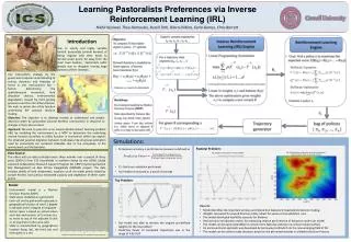
Introduction Due to scanty and highly variable rainfall, pastoralists (animal herders) of Kenya migrate with their herds to remote water points far away from the main town location. Pastoralists suffer greatly due to draughts loosing large portions of their livestock. Any intervention strategy by the government requires understanding of various dynamics and interplay of forces in this environment like – factors determining the spatiotemporal movement, herd allocation choices, environmental degradation caused by herd grazing pressures and the inter-tribal violence. We wish to derive the utility function underlining the pastoral decision making. Objective:The objective is to develop models to understand and predict decisions taken by pastoralists (animal herders) communities in response to changes in their environment. Approach: We seek to pose this as an Inverse Reinforcement Learning problem (IRL) by modeling the environment as a MDP to determine the underlying reward function (corollary to utility function in economics) which can explain the observed pastoral migration behavior. Techniques like structural estimation used by economists are rendered infeasible due to the complexity of the environment and the behavior. Simulations: Pastoral Problem: • To measure accuracy, a performance measure is defined as Data Source: This effort will use data collected every three months over a period of three years (2000-2) from 150 households in northern Kenya by the USAID Global Livestock Collaborative Research Support Program (GL CRSP) Improving Pastoral Risk Management on East African Rangelands (PARIMA) project. The data includes details of herd movements, locations of all the water points visited by sample herders each period, estimated capacity and vegetation of these water points. Fig: Plot for value surface for each cell in gridworld Fig: Weights recovered for actual problem • 15- fold cross validation performed • Toy Problem simulated as a proof of concept Toy Problem: Model: • Environment model is a Markov Decision Process (MDP). • State space modeled as a grid world • Each cell on the grid world represents a geographical location of size 0.1 degree in latitude and 0.1 degree in longitude • Action space is based on actions taken each day and consists of 9 actions (i.e. to move to any of the adjacent 8 cells or to stay there in the same cell). • State is characterized by geographical location (long, lat), the herd size and time spent in a cell. Results: • Low weight for popularity indicates that these herders prefer smaller water points • Herders prefer water points which have a good vegetation • Weights recovered for reward function pretty robust for various cross validation runs • There is a general benefit of being at a water point indicated by high weight • The model developed implicitly accounts for distance • The model can be easily extendible to contain more features and even non-linear reward surface • Our model was able to retrieve the original pre-defined weightsfor the toy problem • Predictive Power of computed trajectories was in the range of 0.92-0.97 Gridworld model with waterpoints, villages & sample trajectories
Model: • Environment model is a Markov Decision Process (MDP). • State space modeled as a grid world • Each cell on the grid world represents a geographical location of size 0.1 degree in latitude and 0.1 degree in longitude • Action space is based on actions taken each day and consists of 9 actions (i.e. to move to any of the adjacent 8 cells or to stay there in the same cell). • State is characterized by geographical location (long, lat), the herd size and time spent in a cell. Gridworld model with waterpoints, villages & sample trajectories Simulations:
Small Stock RoutesDec. 2000 – Nov.2001 An empty streambed during the dry season near Kargi, Kenya. Treating sheep for scrapies (disease) in a boma (corral). A boy goat herder.
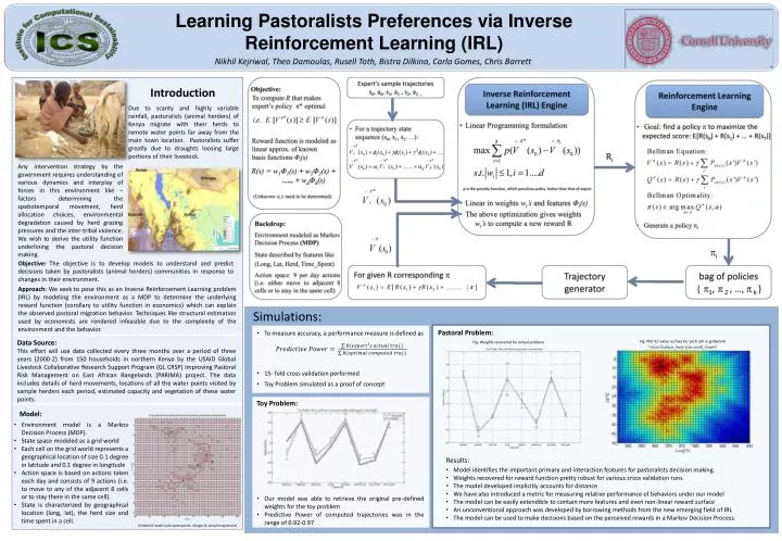
Expert’s sample trajectories • s0, a0, s1, a1 , s2, a2 … Inverse Reinforcement Learning (IRL) Engine • Objective: Reinforcement Learning Engine • To compute R that makes expert’s policy * optimal • Linear Programming formulation • Linear in weights wi’s and features Φi(s) • The above optimization gives weights wi’s to compute a new reward R • Goal: find a policy to maximize the expected score: E[R(s0) + R(s1) + … + R(sT)] • Generate a policy i • For a trajectory state sequence (s0, s1, s2….): • Reward function is modeled as • linear approx. of known • basis functions Φi(s) Ri • R(s) = w1Φ1(s) + w2Φ2(s) + • ….. + wdΦd(s) p is the penalty function, which penalizes policy better than that of expert (Unknown wi’s need to be determined) • Backdrop: • Environment modeled as Markov Decision Process (MDP) i • State described by features like • (Long, Lat, Herd, Time_Spent) • Trajectory generator • bag of policies • { 1, 2 , …, k } For given R corresponding • Action space: 9 per day actions (i.e. either move to adjacent 8 cells or to stay in the same cell)
Reward function is modeled as linear approx. of known basis functions Φi(s) • R(s) = w1Φ1(s) + w2Φ2(s) + ….. + wdΦd(s) (Unknown wi’s need to be determined) • Expert’s sample trajectories • s0, a0, s1, a1 , s2, a2 … Reinforcement Learning Engine Inverse Reinforcement Learning (IRL) Engine • Linear Programming formulation • Linear in weights wi’s and features Φi(s) • The above optimization gives weights wi’s to compute a new reward R • Goal: find a policy to maximize the expected score: E[R(s0) + R(s1) + … + R(sT)] • Generate a policy i • For a trajectory state sequence (s0, s1, s2….): Ri p is the penalty function, which penalizes policy better than that of expert i • Trajectory generator • bag of policies • { 1, 2 , …, k } For sample trajectory under the policy i
Reward function is modeled as linear approximation of some basis functions Φi(s) • R(s) = w1Φ1(s) + w2Φ2(s) + ….. + wdΦd(s) • Unknown wi’s need to be determined • Inverse Reinforcement Learning (IRL) • Goal of standard reinforcement learning(RL) technique is to find a policy which picks actions over time so as to maximize the expected score: E[R(s0) + R(s1) + … + R(sT)] • Goal of IRL is to the reward function R(s) which satisfies the above relation given a policy • For computing R that makes * optimal • Expert policy * is accessible through a set of sampled trajectories and is used to estimate • Assume we have some set of policies { 1,2 , …, k } • Linear Programming formulation • The above optimization gives a new reward R, we then compute k+1 based on R, and add it to the set of policies • reiterate p is the penalty function, which penalizes policy better than that of expert (Andrew Ng & Struat Russell, 2000)
We have been able to generate around 1750 expert trajectories described over a period of 3 months (~90 days) • We have modeled the state space as grid world. Each cell on the grid world represents a particular geographical location of size 0.1 degree in latitude and 0.1 degree in longitude. The action space is based on actions taken each day and consists of 9 actions (i.e. to move to any of the adjacent 8 cells or to stay there in the same cell). • State is uniquely identified by geographical location (long, lat), the herd size and time spent at that water point • S = (Long, Lat, Herd, Time_Spent) • We also decided to go with a Reward function which is linear in features where the features describe a state and can be themselves be non-linear yielding a non-linear reward function. • R(s) = W * [veg, popularity, herd_size, is_waterpoint, time_spent, interaction terms,… interaction_terms];
Simulations To measure accuracy , a performance measure ‘Predictive Power’ is defined as • We simulated a toy problem as a proof concept. • For the toy problem we used exactly the same model with pre-defined the weights of the linear reward. A synthetic generator was then used to generate sample expert trajectories. • Our model was able to retrieve the original weights. • Predictive Power of computed trajectories was in the range of 0.92-0.97 15 fold cross validation is performed to estimate the parameters and final value is average of these 15 values.
Results • Predictive Power for cross validation runs ranged between 0.72- 0.85. Herd size also seems to little effect on overall policy. Low values on popularity shows that these herders prefer water points which are smaller in size. They may be visiting water points which are relatively smaller. Herders prefer water points which have a good vegetation. They pay a lot of importance to vegetation as it is a source of forage for the animals. There is a general benefit of being at a water point, it can be inversely thought as the cost of not being at a water point(i.e. being in some intermediate loaction). So in the model the herders pay a cost each day they are not at a water point.
Inverse Reinforcement Learning Environment Model (MDP) Inverse Reinforcement Learning (IRL) Reward Function R (s) Optimal policy p R that explains expert trajectories Expert Trajectories s0, a0, s1, a1 , s2, a2 …
Simulations: Pastoral Problem: • To measure accuracy, a performance measure is defined as Fig: Plot for value surface for each cell in gridworld Fig: Weights recovered for actual problem • 15- fold cross validation performed • Toy Problem simulated as a proof of concept Toy Problem: Results: • Low weight for popularity indicates that these herders prefer smaller water points • Herders prefer water points which have a good vegetation • Weights recovered for reward function pretty robust for various cross validation runs • There is a general benefit of being at a water point indicated by high weight • The model developed implicitly accounts for distance • The model can be easily extendible to contain more features and even non-linear reward surface • Our model was able to retrieve the original pre-defined weightsfor the toy problem • Predictive Power of computed trajectories was in the range of 0.92-0.97