Download
1 / 25
250 likes | 334 Vues
The AutoSimOA Project aims to provide an easy-to-use method to determine the number of replications needed for accurate results in discrete event simulation models. This project explores different methods such as Rule of Thumb, Graphical Method, Confidence Interval Method, and Prediction Formula for selecting the ideal number of replications. The project proposes an automated Confidence Interval Method algorithm that interacts with the simulation model to calculate the necessary replications for desired precision.

E N D
AUTOMATING D.E.S OUTPUT ANALYSIS: The AutoSimOA Project HOW MANY REPLICATIONS TO RUN Katy Hoad, Stewart Robinson, Ruth Davies Warwick Business School WSC 07 A 3 year, EPSRC funded project in collaboration with SIMUL8 Corporation. http://www.wbs.ac.uk/go/autosimoa
Objective To provide an easy to use method, that can be incorporated into existing simulation software, that enables practitioners to obtain results of a specified accuracy from their discrete event simulation model. (Only looking at analysis of a single scenario)
OUTLINE Introduction Methods in literature Our Algorithm Test Methodology & Results Discussion & Summary
Perform N replications summary statistic from each replication Response measure of interest Underlying Assumptions • Any warm-up problems already dealt with. • Run length (m) decided upon. • Modeller decided to use multiple replications to obtain better estimate of mean performance.
QUESTION IS… How many replications are needed? Limiting factors: computing time and expense. 4 main methods found in the literature for choosing the number of replications N to perform.
Rule of Thumb(Law & McComas 1990) • Run at least 3 to 5 replications. • Advantage: Very simple. • Disadvantage: Does not use characteristics of model output. • No measured precision level.
2. Simple Graphical Method (Robinson 2004) Advantages: Simple Uses output of interest in decision. Disadvantages: Subjective No measured precision level.
3.Confidence Interval Method (Robinson 2004, Law 2007, Banks et al. 2005). Advantages: Uses statistical inference to determine N. Uses output of interest in decision. Provides specified precision. Disadvantage:Many simulation users do not have the skills to apply approach.
4.Prediction Formula (Banks et al. 2005) • Decide size of error εthat can be can tolerated. • Run ≥ 2 replications - estimate variance s2. • Solve to predict N. • Check desired precision achieved – if not recalculate N with new estimate of variance. Advantages: Uses statistical inference to determine N. Uses output of interest in decision. Provides specified precision. Disadvantage:Can be very inaccurate especially for small number of replications.
AUTOMATE Confidence Interval Method:Algorithm interacts with simulation model sequentially.
We define the precision, dn, as the ½ width of the Confidence Interval expressed as a percentage of the cumulative mean: Where n is the current number of replications carried out, is the student t value for n-1 df and a significance of 1-α, is the cumulative mean, snis the estimate of the standard deviation, calculated using results Xi (i = 1 to n) of the n current replications. ALGORITHM DEFINITIONS
Stopping Criteria • Simplest method: Stop when dn 1st found to be ≤ desired precision, drequired . Recommend that number of replications, Nsol, to user. • Problem: Data series could prematurely converge, by chance, to incorrect estimate of the mean, with precision drequired , then diverge again. • ‘Look-ahead’ procedure: When dn 1st found to be ≤ drequired, algorithm performs set number of extra replications, to check that precision remains ≤ drequired.
‘Look-ahead’ procedure kLimit = ‘look ahead’ value. Actual number of replications checked ahead is Relates ‘look ahead’ period length with current value of n.
Replication Algorithm 95% confidence limits Precision ≤ 5% Cumulative mean, f(kLimit) Nsol + f(kLimit) Nsol
Precision ≤ 5% Precision > 5% Precision ≤ 5% f(kLimit) Nsol2 + f(kLimit) Nsol2 Nsol1
TESTING METHODOLOGY • 24 artificial data sets: Left skewed, symmetric, right skewed; Varying values of relative st.dev (st.dev/mean). • 100 sequences of 2000 data values. • 8 real models selected. • Different lengths of ‘look ahead’ period tested: kLimit values = 0 (i.e. no ‘look ahead’), 5, 10, 25. • drequiredvalue kept constant at 5%.
5 performance measures • Coverage of the true mean • Bias • Absolute Bias • Average Nsol value • Comparison of 4. with Theoretical Nsol value • For real models: ‘true’ mean & variance values - estimated from whole sets of output data (3000 to 11000 data points).
Results • Nsol values for individual algorithm runs are very variable. • Average Nsol values for 100 runs per model close to the theoretical values of Nsol. • Normality assumption appears robust. • Using a ‘look ahead’ period improves performance of the algorithm.
Impact of different look ahead periods on performance of algorithm
Examples of changes in Nsol & improvement in estimate of true mean
DISCUSSION • kLimit default value set to 5. • Initial number of replications set to 3. • Multiple response variables - Algorithm run with each response - use maximum estimated value for Nsol. • Different scenarios - advisable to repeat algorithm every few scenarios to check that precision has not degraded significantly. • Implementation into Simul8 simulation package.
SUMMARY • Selection and automation of Confidence Interval Method for estimating the number of replications to be run in a simulation. • Algorithm created with ‘look ahead’ period -efficient and performs well on wide selection of artificial and real model output. • ‘Black box’ - fully automated and does not require user intervention.
Thank you for listening. ACKNOWLEDGMENTSThis work is part of the Automating Simulation Output Analysis (AutoSimOA) project (http://www.wbs.ac.uk/go/autosimoa) that is funded by the UK Engineering and Physical Sciences Research Council (EP/D033640/1). The work is being carried out in collaboration with SIMUL8 Corporation, who are also providing sponsorship for the project. Katy Hoad, Stewart Robinson, Ruth Davies Warwick Business School WSC 07