Download
1 / 69
690 likes | 878 Vues
El Ni ñ o, La Ni ñ a and Southern Oscillation: A Climate Variability arising from coupling between the Atmosphere and the Ocean B. N. Goswami Centre for Atmospheric and Oceanic Sciences Indian Institute of Science.

E N D
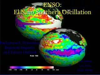
El Niño, La Niña and Southern Oscillation: A Climate Variability arising from coupling between the Atmosphere and the Ocean B. N. Goswami Centre for Atmospheric and Oceanic Sciences Indian Institute of Science
For many years, coastal residents of Peru had noticed a strange feature of the eastern Pacific Ocean waters that border their home. This region of tropical yet relatively cool water is host to one of the world's most productive fisheries and a large bird population. In the first months of each year, a warm southward current usually modified the cool waters (Fig.1). But every few years, this warming started early (in December), was far stronger, and lasted as long as a year or two (Fig.2). Torrential rains fell on the arid land; as one early observer put it, "the desert becomes a garden." Warm waters flowing south brought water snakes, bananas, and coconuts from equatorial rain forests. However, the same current shut off the deeper, cooler waters that are crucial to sustaining the region's marine life and drastic reduction in fish catch (Fig.3).
Time series of Anchovy catch in Peru and Guano birds population.
This is El Niño, "the Christ child," so named because of its frequent late December appearance. Once thought to affect only a narrow strip of water off Peru, it is now recognized as a large-scale oceanic warming that affects most of the tropical Pacific. The meteorological effects related to El Niño and its counterpart, La Niña (a cooling of the eastern tropical Pacific), extend throughout the Pacific Rim to eastern Africa and beyond. El Niño is normally accompanied by a change in atmospheric circulation called the Southern Oscillation. Together, the ENSO (El Niño - Southern Oscillation) phenomenon is one of the main sources of interannual variability in weather and climate around the world. For example, it produces flooding in north western America and forest fires in Indonesia.
Since recognizing some 25 years ago that the oceanic and atmospheric parts of ENSO are strongly linked, scientists have moved steadily toward a deeper understanding of ENSO. Climate forecasters have taken the first steps toward predicting the onset of El Niño and La Niña events months in advance. Still, much remains to be learned about these children of the tropics. • Examples of two recent El Nino Events • SST and anomaly during 1982/83 • SST and anomaly during 1987/98
Ocean and Atmospheric Changes associated with El Nino and La Nina
Sea-Saw of sea level pressure associated with El Niño and La Niña is shown. During an El Niño the sea level pressure in the east Pacific decrease while that over west Pacific and Indonesia increases. In a La Niña it is higher pressure in the east and lower pressure in the west.
Animation of SST anomalies from January 1982-December 1983 Restart Animation Anomaly = (Current Observation - Corresponding Climatological Value)Base period for the climatology is 1950-1979 Anomaly = (Current Observation - Corresponding Climatological Value)Base period for the climatology is 1950-1979
Animation of SST anomalies from January 1997-December 1998 Anomaly = (Current Observation - Corresponding Climatological Value)Base period for the climatology is 1950-1979
Next figure depicts a sequence of longitude-depth cross-sections of mean temperature in the equatorial Pacific Ocean for the months from January 1997 to May 1998. This period corresponds to the onset and intensification of the 1997-98 El Nino event. Clearly evident in Figure is the normal pooling of very warm water and the depression of the thermocline in the western Pacific in January 1997, and the eastward march of warmer than normal temperatures (positive temperature anomalies) from this region during the 1997-98 El Nino event. Notice the extensive cap of exceptionally warm surface waters in the eastern Pacific in January of 1998, the tell-tale signal of the arrival of El Nino in the Pacific coastal waters of equatorial South America. One can well imagine that the presence of this abnormally warm water profoundly influences and interferes with the normal upwelling of cold deep water and the delivery of life-sustaining nutrients to the base of the marine food chain. It is interesting to note that a large pool of subsurface cold water formed in the western Pacific in January 1998, when the El Nino was in its peak in the eastern Pacific.
The sea-level pressure difference between Darwin and Tahiti can be used as an index of the SO (SOI)and, by extension, as a guide to the major ENSO events of the past. Next figure shows the SOI anomalies (deviations above or below normal) of the past half century, smoothed to eliminate short-term effects together with SST anomalies over Nino-3 area (160W-90W, 5S-5N). Note that • The SST variations are strongly correlated with the pressure seesaw. • El Nino and La Nina events tend to alternate about every three to seven years. However, the time from one event to the next can vary from one to ten years. • The strength of the events, as judged by the SOI anomaly or Nino-3 anomaly, varies greatly from case to case. The strongest El Ninos in this record occurred in 1982-83 and 1997-98 (The effects of 1982-1983 included torrential storms throughout the southwest United States and Australia's worst drought this century. • Sometimes El Nino and La Nina events are separated not by their counterparts, but by rather normal conditions.
Normalized time series of SST anomalies over Nino 3 area (blue) and Southern Oscillation Index (SOI, red).
The above figure and other evidence like it reveals that ENSO is a quasi-periodic yet highly variable phenomenon. Sometimes the warm waters generated by an El Nino flow all the way across the Pacific. The 1997-98 event increased surface water temperatures near Peru by 5ºC (9ºF). In the much weaker event of 1986-87, the warm water extended eastward only as far the mid-Pacific (near 170W) and raised the temperatures there a modest 1ºC (1.8ºF) or so. In still other cases, warm anomalies first appear offshore of Peru and then progress westward to meet the preexisting warm pool. Global Climatic Impacts of ENSO
Frequency of occurrence of Jun-Nov (rainy season) rainfall anomaly in 20 El Nino years and 20 La Nina years during 100 year record of rainfall in Indonesia. If all years are taken together, the distribution is Gaussian. El Nino years are characterized by above normal rainfall while the La Nina years are by below normal rainfall.
Departure of all India seasonal rainfall from long term mean normalized by its own standard deviation. El Nino years are marked blue. A tendency of below normal rainfall to occur with El Nino may be noted. Thin solid line shows 11 year running mean.
Rough estimate of damage around the globe during 1982-83 El Nino.
Understanding the ENSO phenomenon… • To understand these unusual events, let us first examine the normal (mean) conditions in the Pacific. • Mean surface winds during winter • Mean SST during winter • Mean structure of thermocline in the equatorial Pacific
Annual mean SST (top) and vertical cross section of temperature along the equator
The persistent easterly trade winds are a key ingredient in the ENSO process. They have two major effects: • Pushing water toward the western Pacific. The sea level in the Philippines is normally about 60 centimeters (23 inches) higher than the sea level on the southern coast of Panama. • Allowing the westward-flowing water to remain near the surface and gradually heat. This gives the water's destination-the western Pacific-the warmest ocean surface on Earth. Usually above 28ºC (82ºF), parts of this pool are sometimes as warm as 31.5ºC (89ºF). • As warm surface water collects in the western Pacific, it tends to push down the thermocline, the boundary separating well-mixed surface waters from deeper, colder waters. The thermocline is usually about 40 meters (130 feet) deep in the eastern Pacific but varies from 100 to 200 meters (330-660 feet) deep in the west.
The clearest sign of the SO is the inverse relationship between surface air pressure at two sites: Darwin, Australia, and the South Pacific island of Tahiti. As seen in Figure 1, high pressure at one site is almost always concurrent with low pressure at the other, and vice versa. The pattern reverses every few years. It represents a standing wave or "see-saw", a mass of air oscillating back and forth across the International Date Line in the tropics and subtropics. This two-dimensional picture was extended vertically by renowned meteorologist Jacob Bjerknes in 1969. He noted that trade winds across the tropical Pacific flow from east to west. To complete the loop, he theorized, air must rise above the western Pacific, flow back east at high altitudes, then descend over the eastern Pacific. Bjerknes called this the Walker circulation (in honor of Sir Gilbert Walker); he also was the first to recognize that it was intimately connected to the oceanic changes of El Nino and La Nina.
How the mean state of the ocean and the atmosphere change during El Nino and La Nina are schematically shown
Bjerknes Hypothesis Renowned meteorologist Jacob Bjerknes suggested in 1969 that the mean ocean and atmospheric circulation as well as the ENSO result from true coupling between the atmosphere and the ocean. The persistent oceanic heat surrounding Indonesia and other western-Pacific islands leads to frequent thunderstorms and some of the heaviest rainfall on Earth. The rainfall is abetted by the upward motion produced by the Walker circulation. The distribution of SSTs drives the enhanced rainfall, Walker circulation, and associated trade winds, which in turn are responsible for the ocean currents and the distribution of SSTs. The atmosphere drives the ocean and the ocean drives the atmosphere in a truly coupled mode of behavior. This coupling is schematically shown in Figure.
Due to some perturbation (such as an westerly wind burst), if the easterly wind weakens in the western Pacific, it could not maintain the pressure gradient and warm water would flow as a Kelvin wave pulse to the east. Warmer water to the east causes atmospheric response with westerly wind anomaly to the west and further weaken the trade winds. More warm water would flow to the east. This unstable air-sea interaction could lead to an El Nino. Bjerknes had no idea how the unstable situation comes back to normal and goes to a La Nina situation. We shall come back to this point little later. First let us summarize some evidence that establishes that there is coupling between the atmosphere and the Ocean. Then we shall review theoretically how coupling could lead to an unstable mode of oscillation.
SST anomaly over Nino-3 area (blue) normalized by its s.d. and SOI (Darwin-Tahiti SLP) also normalized by its own s.d.
Air-sea interaction theory of ENSO How does atmosphere and ocean interact in the tropics? Changes in SST Ts Changes in evaporation Es Changes in atmospheric heating Q Surface stress drives ocean currents Changes in atmospheric circulation C (surface stress)