Download
1 / 31
310 likes | 606 Vues
A radiative transfer framework for rendering materials with anisotropic structure. Wenzel Jakob * Adam Arbree § Jonathan T. Moon † Kavita Bala * Steve Marschner * * Cornell University § Autodesk † Google Modified from the original slides. Wood photograph. Wood micrograph.

E N D
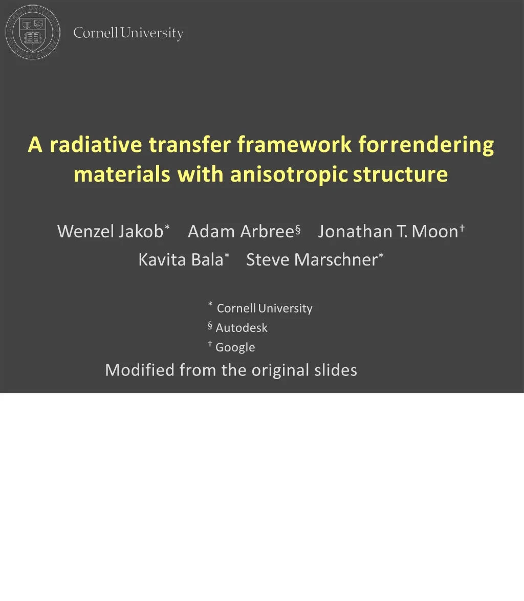
A radiative transfer framework forrendering materials with anisotropicstructure WenzelJakob* AdamArbree§ JonathanT.Moon† KavitaBala* SteveMarschner* * CornellUniversity §Autodesk †Google Modified from the original slides
Woodphotograph Woodmicrograph [Marschner etal.] [NC Brown Center for UltrastructureStudies] Animalfur Moss [Wikimediacommons] [Wikimediacommons] Here’s a sample of several interesting types of materials. Common to all of them is their complex internal structure, which has a profound influence on their appearance. In this talk, I’m going to present a principled way to render such materials using a unified volumetric formulation.
Woodphotograph Woodmicrograph Animalfur Moss [Marschner etal.] [NC Brown Center for UltrastructureStudies] [Wikimediacommons] [Wikimediacommons] • Anisotropicvolumes • Objects with suitable volumetricrepresentations • Anisotropy caused by internalstructure • Current theory doesn’t handlethis! For objects of such vast geometric detail, its preferable to consider them as volumes. We’re interested in anisotropic materials whose internal structure causes them to reflect light differently depending on the directions, from which they are illuminated andobserved. Currently however, when you mix radiative transfer and anisotropy, things begin to break. So we need a way to combine thesetwo.
Twodisjointapproachesforrenderingvolumes: [Fedkiw etal.] [Wikipediacommons.] • Physicallybased radiativetransfer • Soundfoundation • Inherentlyisotropic • Heuristicmodels volumevisualization • Supportanisotropy • Not suitable for multiplescattering And then there is what could be described as volume visualization with heuristic scattering models. For example, medical renderings of volumes often use surface shading models that, in the context of volume scattering, are actually anisotropic. But their heuristic nature prevents them from being usable in full volumetric light transport simulations.
Isotropicscattering Limitations of previoussystems Let’s nowclarifysometerminologyandlimitationsofprevioussystems. Currently, the common convention is to call completely uniform scattering “isotropic”.Thebluepointhereindicatesascatteringinteraction,andthelarge arrowistheincidentdirectionIntheuniformcase,nothingchangeswhenthe incident directionmoves.
Isotropicscattering Limitations of previoussystems “Anisotropic”scattering • Good enoughfor: • Smoke,steam • Cloud of randomly oriented icecrystals Moregeneralformsofscatteringwherethescatteredenergydependsonthe angle between the incident and outgoing directions have traditionally been referred to as“anisotropic”. This is good enough to handle things like a cloud of steam !lled with spherical water droplets. And it even extends to things like a cloud !lled with non- spherical ice crystals, assuming that they are allrandomlyoriented. Butthemain limitation commontobothofthesecasesisthatthemediummustalways behavethesamewayindependentlyofthedirectionofpropagation,whichif youthinkaboutitisreallythede!nitionofthetermisotropic.Soinourpaper,we actually refer to both of them asisotropic.
Isotropicscattering Limitations of previoussystems Isotropic “Anisotropic”scattering Built-inassumption: The medium behaves the same independently of the directionof propagation. Moregeneralformsofscatteringwherethescatteredenergydependsonthe angle between the incident and outgoing directions have traditionally been referred to as“anisotropic”. This is good enough to handle things like a cloud of steam !lled with spherical water droplets. And it even extends to things like a cloud !lled with non- spherical ice crystals, assuming that they are allrandomlyoriented. Butthemain limitation commontobothofthesecasesisthatthemediummustalways behavethesamewayindependentlyofthedirectionofpropagation,whichif youthinkaboutitisreallythede!nitionofthetermisotropic.Soinourpaper,we actually refer to both of them asisotropic.
Anisotropicscattering • Cloud of aligned icecrystals • Cloth fibers, wood,.. Incomparison,wewanttobeabletohandlematerialslikecloth!bersorwood, wherethescatteringbehaviordoesdependonthedirectionofpropagation. It’s a good question to ask if we can use scattering models like these together withtheexistingequations.Hopefully,bytheendofthistalk,youwillagreewith methatifyoudothis,thenthingswillbreakinsubtleandunanticipatedways.
Equations SolutionTechniques Radiative transfer equation Contributions Models Here is an outline of the talk: We’ll start by making a modification to the radiative transfer equation, which leads to an anisotropic form. Before we’re able to start rendering using Monte Carlo techniques, we still need a suitable scattering model, and here we propose one that is based on specularly reflectingflakes. One common approximation that can be derived now is the diffusionapprox. But because our earlier changes propagate, it takes on a new anisotropic form. We also adapt two associated diffusion-based solution techniques to suit this new equation. Due to the time limitations, we can only give a very high-level overview of these steps, and we refer you to the paper and technical report fordetails.
Equations SolutionTechniques Anisotropicradiative transferequation Radiativetransfer equation Contributions Models Here is an outline of the talk: We’ll start by making a modification to the radiative transfer equation, which leads to an anisotropic form. Before we’re able to start rendering using Monte Carlo techniques, we still need a suitable scattering model, and here we propose one that is based on specularly reflectingflakes. One common approximation that can be derived now is the diffusionapprox. But because our earlier changes propagate, it takes on a new anisotropic form. We also adapt two associated diffusion-based solution techniques to suit this new equation. Due to the time limitations, we can only give a very high-level overview of these steps, and we refer you to the paper and technical report fordetails.
Equations SolutionTechniques Anisotropicradiative transferequation Radiativetransfer equation Contributions Models Micro-flake scatteringmodel MonteCarlo Here is an outline of the talk: We’ll start by making a modification to the radiative transfer equation, which leads to an anisotropic form. Before we’re able to start rendering using Monte Carlo techniques, we still need a suitable scattering model, and here we propose one that is based on specularly reflectingflakes. One common approximation that can be derived now is the diffusionapprox. But because our earlier changes propagate, it takes on a new anisotropic form. We also adapt two associated diffusion-based solution techniques to suit this new equation. Due to the time limitations, we can only give a very high-level overview of these steps, and we refer you to the paper and technical report fordetails.
Equations SolutionTechniques Anisotropicradiative transferequation Radiativetransfer equation Contributions Models Micro-flake scatteringmodel MonteCarlo Anisotropicdiffusion approximation Diffusion approximation Anisotropicdipole FiniteElement Method Here is an outline of the talk: We’ll start by making a modification to the radiative transfer equation, which leads to an anisotropic form. Before we’re able to start rendering using Monte Carlo techniques, we still need a suitable scattering model, and here we propose one that is based on specularly reflectingflakes. One common approximation that can be derived now is the diffusionapprox. But because our earlier changes propagate, it takes on a new anisotropic form. We also adapt two associated diffusion-based solution techniques to suit this new equation. Due to the time limitations, we can only give a very high-level overview of these steps, and we refer you to the paper and technical report fordetails.
Radiative transferequation (spatial dependence dropped forreadability) This is the form in which it is usually written down in computer graphics.
Isotropicform: Radiative transferequation localchange extinction in-scattering source Anisotropicform: localchange extinction in-scattering source (spatial dependence dropped forreadability) Let’s take a look how this equation changes in the anisotropic case, which is shown at the bottom here. You can see that the extinction and scattering coefficients now have a directional dependence, and that the phase function is a proper function of two directions, as opposed to just the angle betweenthem. It’s a really bad idea to just stick some arbitrary functions sigma_s, sigma_t and f sub p into this equation because, they are in fact all related to each other. To find out what these relations are, it necessary to take a step back and derive this equation from first principles. For radiative transfer, this means that we need to reason about the particles that make up the volume. We won’t have time to see how this derivation works in detail, but we can take a look at the ingredients. One general thing to note here is that the material might actually not be made of particles. Despite that, the particle abstraction has proven itself in thepast.
Need several pieces ofinformation: Particledistribution Projectedarea Albedo Phasefunction Particledescription 20% 40% 26% 30% The goal here is to find a compact way of fully characterizing the underlying particles. We do this using several pieces ofinformation: First, we need a density function that tells us how the particles are distributed both spatially anddirectionally. Secondly, we need to know how much light a particle intercepts– so we need a function that tells us the projected area from 6% 30 The particle might reflect different amounts of light depending on the direction from which it is illuminated, so we need to provide a directionally varying albedofunction. different directions. And each particle itself also has a phase function that determines the scattered direction after an interaction takesplace.
Need several pieces ofinformation: Particledistribution Projectedarea Albedo Phasefunction Particledescription 20% 40% 26% 30% the paper provides a way of determining what the volume’s scattering coefficients and the phase function shouldbe.
Example: extinctioncoefficient projected areafunction particledistribution All of them turn into integrals over the sphere. The easiest one is the extinction coefficient, which is simply the convolution of the projected area function of a single particle with the particle distribution. This means that the amount of extinction can potentially vary quite strongly with the direction of propagation, and here is a just picture to illustratethat.
Models Equations SolutionTechniques Anisotropicradiative transferequation Radiativetransfer equation Micro-flake scatteringmodel MonteCarlo Anisotropicdiffusion approximation Diffusion approximation Anisotropicdipole FiniteElement Method So now we have this equation to work with — but by itself we can’t use it yet. The reason for this is simply that nobody has ever used this anisotropic RTE before, so there are no scattering models for it. To fix this, we propose a new model called “micro-flakes”. One thing to note here is that this is not a restriction -- most of the paper is equally applicable if you’d rather come up with your ownmodel.
Approach • Plugs into the discussed particleabstraction • Simple ideal mirror-like reflector on bothsides Micro-flakes surfacestructure flakedistribution We present a simple model inspired by microfacet models, which turns out to get you pretty far. It’s based on little flakes with ideal mirror-like reflection on both sides. These plug directly into the earlier particle abstraction, which gives you scattering coefficients and a phasefunction. We use flakes to simulate various materials, even if they aren’t actually made out of flakes in real-life. We mainly consider them to be a flexible tool for expressing different types of scattering, but without necessarily implying a specific internal makeup of yourmaterial. The next question is: how do we choose the particle distributions. This decision is guided by the type of reflection we want our volume torepresent. For instance, to make a volume behave similarly to a rough surface, we choose the flake distribution on the right side here shown as a polar plot over the flake normals. Because most point upwards, the volume behaves like a translucent rough surface, which is oriented in that direction. Another way to think about this is as chopping up a facet representation of a surface and then building a histogram over the observednormals.
Approach • Plugs into the discussed particleabstraction • Simple ideal mirror-like reflector on bothsides Micro-flakes surfacestructure flakedistribution And to make volume region behave like a rough fiber, we choose a “fibrous” equatorial flake distribution using the sameprinciple.
Approach • Plugs into the discussed particleabstraction • Simple ideal mirror-like reflector on bothsides • Properties • Modelsubsumestraditional“anisotropic”scattering • Leads to analytic results lateron • Half-angleformulation Micro-flakes Some more useful facts: First, this model is general enough subsume all traditional volume scattering models. So if you wanted to imitate Mie scattering using flakes, then you can find a specific type flake that will behave exactly the sameway. Another motivation for this model is that it leads to analytic solutions later on, when passing from the radiative transfer interpretation to that of anisotropicdiffusion. And finally, it results in a half-angle formulation, which is often a desirableproperty.
Models Equations SolutionTechniques Anisotropicradiative transferequation Radiativetransfer equation Micro-flake scatteringmodel MonteCarlo Anisotropicdiffusion approximation Diffusion approximation Anisotropicdipole FiniteElement Method Having having seen the equations and the model we use, we’ll now take a look at the three solution techniques that can be used to render images of thesematerials.
Changes • Must account for the directional dependence ofthe scatteringcoefficients • Need goodimportance sampling support for the anisotropic phasefunction Solution technique 1: MonteCarlo The most accurate, but the slowest is Monte Carlo, and just few changes are required for this method. What does need to be addressed is that the scattering coefficients are not constants anymore, so they often need to be evaluated with respect to direction. Also, for highly scattering anisotropic media, it is important to have a good way of importance sampling the phase function, otherwise there will just be too much noise. The paper contains some information on how to solve theseproblems. Here are some renderings made using MonteCarlo:
415 Mvoxels 3 GB storage Render time: 5hrs This is a high resolution scarf model represented as a 415 megavoxel volume. At every point in the medium, it contains both a density value and a local fiber orientation. The blue glow is completely due to multiple scattering. We would expect small highlights to run along the plies that make up the yarn, but because the rendering seen here is isotropic, the image looks a bit dull, and the illumination is relatively washedout. But if we use the stored fiber orientations to define micro-flake distributions of the equatorial type at every point in the medium, we can switch to the anisotropic form of the radiative transfer equation and create thisimage:
415 Mvoxels 3 GB storage Render time: 22hrs Here is an animatedcomparison
As you can see, accounting for the anisotropic structure leads to a significantly changed appearance, including much more realistic highlights. Up to now, physically based renderings of this kind have not beenpossible. We have also made some experiments with the captured wood fiber orientations from the 2005 SIGGRAPH paper on finishedwood.
That paper contained a *completely* specialized model that was only suitable for wood, and it also contained an ad-hoc diffusecomponent. We tried to reproduce the shifting highlights observed in that work, but now using the much more general micro-flakes and multiplescattering.
And even though the flakes really weren’t made with wood in mind, this turns out to work, and we automatically get things like get energy conservation and reciprocity forfree.
We also projected some very bright parallel beams onto the same slab, and we see these interesting spatially varying diffusion effects along the grain direction of the wood. This is something that the original model wouldn’t have been able todo. One downside to the Monte Carlo approach is that all of these images take a really long time to render, from a few hours to almost a day. To improve on that, we’ll take a look at the FEMsolver:
Contributions • Principled foundation for work on complexmaterials • Theory: Anisotropic RTE, Anisotropic diffusionequation • Model: Micro-flake scatteringmodel • Solution techniques: Monte Carlo, FEM,Dipole Implications and futurework In conclusion, this paper provides end-to-end derivation of the changes required to support anisotropy in current volume rendering systems. First and foremost, we believe that this framework can provide a solid foundation for a principled and powerful new way of thinking about complex materials that couldn’t be handled in the past. The derivations led to two new equations, a modified radiative transfer equation and a generalized anisotropic form of the diffusion equation. To use these equations in practice, we proposed a new scattering model, and we showed how to then solve them using three different solutiontechniques.
Contributions • Principled foundation for work on complexmaterials • Theory: Anisotropic RTE, Anisotropic diffusionequation • Model: Micro-flake scatteringmodel • Solution techniques: Monte Carlo, FEM,Dipole • Futurework • Level of detail(LoD) • Bidirectional renderingschemes • Fitting of micro-flakedistributions Implications and futurework There are several directions for future work we have inmind: One is to use this framework to do volume level of detail correctly. The challenge is that volumes generally start to become increasingly anisotropic as you look at larger regions, even if you initially started out with something isotropic. We would also like to investigate integration with bidirectional rendering schemes like Metropolis LightTransport. And finally, another question is just how expressive the flake model is. As with microfacet models, it certainly cannot represent any kind of scattering, so it’ll be interesting to explore the underlying limitations a bit more, and to use it to fit existingdata.