2. The classification of physical quantities

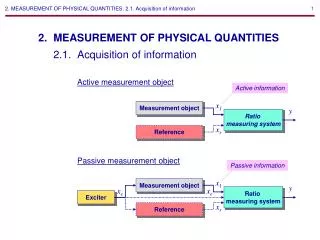
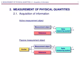
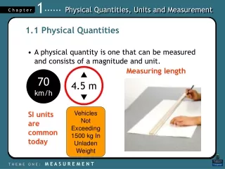
2. 2. The classification of physical quantities Physical quantities are classified according to several criteria: 1. In direction. The physical quantity that reflects the direction of motion, called vector quantity, otherwise scalar quantity. 2. By the character of dimension. The physical quantity which has dimension formula, in which at least one dimension of a non-zero exponent, called dimensional quantity. If all dimensions have a zero exponent, then this quantity called dimensionless quantity. International Vocabulary of Metrology JCGM 200:2012 allows the use by the term "dimensionless quantity" only for historical reasons, but recommended to prefer the term "quantity of dimension one". 3. If possible summation. The physical quantity is called the additive quantity, if its values ​​can be summarized, multiplied by a numerical factor, divided against each other, as, for example, that can be done with the force or moment of force, and non-additive quantity, if the mathematical operations have no physical meaning, such as a thermodynamic temperature whose value does not make sense to add or subtract. 4. With respect to the of a physical quantity physical system. The physical quantity is called extensive quantity, if its value is the sum of the values ​​of the same physical quantities for subsystems of which comprises a system such as that of volume and intensive quantity, if its value does not depend on the size of the system, such as in thermodynamic temperature.

4. Carnap Criteria Rudolf Carnap(1891 – 1970) German-born philosopher For any quantity, a competentmetrologist with suitable equipment is one who has a realization of fouraxiom: 1. Within the domain of objects accessible one object must be the unit 2. Within the domain of objects accessible one object must be zero 3. There must be a realizable operation to order the objectsas to magnitude or intensity of the measured quantity. 4. There must be an algorithm to generate a scale betweenzero and the unit To make the above clear, consider the following system: • The quantity of interest, temperature; • the object, a human body; • the unit, the boiling point of water 100°; • the zero, the triple point of water 0°; • the ordering operator, the height of a mercury columnin a uniform bore tubing connected to a reservoircapable of being placed in a body cavity; • the scale, shall be a linear subdivision between theheights of the column when in equilibrium with boilingwater and water at the triple point

5. Temperature:linear scale But pH scale is logarithmic!

6. Math and science were invented by humans to describe and understand the world around us. We live in a (at least) four-dimensional world governed by the passing of time and three space dimensions; up and down, left and right, and back and forth. We observe that there are some quantities and processes in our world that depend on the direction in which they occur, and there are some quantities that do not depend on direction. For example, the volume of an object, the three-dimensional space that an object occupies, does not depend on direction.

7. Frame of reference Motion (or other property) of a body is always described with reference to some well defined coordinate system. This coordinate system is referred to as 'frame of reference'. In three dimensional space a frame of reference consists of three mutually perpendicular lines called 'axes of frame of reference' meeting at a single point or origin.The coordinates of the origin are O(0,0,0) and that of any other point 'P' in space are P(x,y,z).The line joining the points O and P is called the position vector of the point P with respect to O.

9. Frame of referenceexample

11. Frame of Reference Transformations Reflection Translation Rotation

12. Tensor Any tensor with respect to a basis is represented by a multidimensional array. For example, a linear operator is represented in a basis as a two-dimensional square n × n array. The numbers in the multidimensional array are known as the scalar components of the tensor or simply its components. They are denoted by indices giving their position in the array, as subscripts and superscripts, following the symbolic name of the tensor. For example, the components of an order 2 tensor T could be denoted Tij , where i and j are indices running from 1 to n, or also by Tij. Whether an index is displayed as a superscript or subscript depends on the transformation properties of the tensor, described below. The total number of indices required to identify each component uniquely is equal to the dimension of the array, and is called the order, degree or rank of the tensor. However, the term "rank" generally has another meaning in the context of matrices and tensors.

13. Properties of scalar, vector and tensor quantities for coordinate transformations

14. Vector calculus - basics A vector – standard notation for three dimensions Unit vectors i,j,kare vectors of magnitude 1 in directions of the x,y,z axes. Magnitude of a vector Position vector is a vector r from the origin to the current position where x,y,z, are projections of r to the coordinate axes.

15. Adding and subtracting vectors Multiplying a vector by a scalar Example of multiplying of a vector by a scalar in a plane

16. Example of addition of three vectors in a plane The vectors are given: Numerical addition gives us Graphical solution:

17. Example of subtraction of two vectors a plane The vectors are given: Numerical subtraction gives us Graphical solution:

18. Scalar product Scalar product (dot product) – is defined as Where Θ is a smaller angle between vectors a and b and S is a resulting scalar. For three component vectors we can write Geometric interpretation – scalar product is equal to the area of rectangle havinga and b.cosΘas sides.Blue and red arrows represent original vectors a and b. Basic properties of the scalar product

19. Vector product Vector product (cross product) – is defined as Where Θ is the smaller angle between vectors a and b and n is unit vector perpendicular to the plane containing a and b. Geometric interpretation - the magnitude of the cross product can be interpreted as the positive area Aof the parallelogram having a and b as sides Component notation Basic properties of the vector product

20. Direction of the resulting vector of the vector productcan be determined eitherby the right hand rule or by the screw rule Vector triple product Geometric interpretation of the scalar triple product isa volume of a paralellepipedV Scalar triple product

21. Operatorsin scalar and vector fields • gradient of a scalar field • divergence of a vector field • curl of a vector field

22. GRADIENT OF A SCALAR FIELD We will denote by f(M) a real function of a point Min an area A. If A is two dimensional, then and, if A is a 3-D area, then We will call f(M) a scalar field defined in A.

23. Let f(M) = f(x,y). Consider an equation f(M) = c. The curve defined by this equation is called a level line (contour line, height line) of the scalar field f(M). For different values c1, c2, c3, ... we may get a set of level lines. y x c5 c4 c3 c2 c1

24. Similarly, if A is a 3-D area, the equation f(M) = c defines a surface called a level surface (contour surface). Again, for different values of c, we will obtain a set of level surfaces. z c1 c2 c3 y c4 x

25. Scalar fields – Magnitudes • Temperature • Pressure • Gravity anomaly • Resistivity • Elevation • Maximum wind speed (without directional info) • Energy • Potential • Density • Time…

26. Scalarfieldexample: Temperaturedistributionin a multitubularreactor

27. Scalarfieldexample #2: Heatexchangers

28. Directional derivative Let F(M) be a 3-D scalar field and let us construct a value that characterizes the rate of change of F(M) at a point M in a direction given by the vector e = (cos , cos , cos ) (the direction cosines). z M1 M y x

29. Let M = [x,y,z] and M1=[x+x, y+y, z+z], then and as where

30. This gives us However, the first three terms of the limit do not depend on  and so that

31. Clearly, assumes its greatest value for This vector is called the gradient of F denoted by or, using the Hamiltonian operator

32. z y x Thus grad F points in the direction of the steepest increase in F or the steepest slope of F. Geometrically, for a c, grad F at a point M is parallel the unit normal n at M of the level surface grad F n M

33. Scalar field and gradient Scalar fieldassociates a scalar quantity to every point in a space. This association can be described by a scalar function fand can be also time dependent. (for instance temperature, density or pressure distribution). The gradient of a scalar field is a vector field that points in the direction of the greatest rate of increase of the scalar field, and whose magnitude is that rate of increase. Example: the gradient of the function f(x,y) = −(cos2x + cos2y)2 depicted as a projected vector field on the bottom plane.

34. Example 2 – finding extremes of the scalar field Find extremes ofthe function: Extremes can be found by assuming: In this case : Answer: there are two extremes

35. Vector operators Gradient (Nabla operator) Divergence Curl Laplacian

36. Vector field, vector lines Let a vector field f(M) be given in a 3-D area , that is, each is assigned the vector A vector linel of the vector field f(M) is defined as a line with the property that the tangent vector to l at any point L of l is equal to f(L).

37. Vector fields – Magnitude and direction • Includes displacement, velocity, acceleration, force, momentum… • Magnetic field (Scale Earth or mineral) • Water velocity field • Wind direction on a weather map • Electric field

38. Vector fields VELOCITY FIELDS The speed at any given point is indicated by the length of the arrow.

39. This means that if we denote by the tangent vector of l,then, at each point M, the following equations hold This yields a system of two differential equations that can be used to define the vector lines for f(M). This system has a unique solution if f1, f2, f3 together with their first order partial derivatives are continuous and do not vanish at the same point in . Then, through each , there passes exactly one vector line. Note: For a two-dimensional vector field we similarly get the differential equation

40. Example Find the vector line for the vector field passing through the point M = [1, -1, 2]. Solution We get the following system of differential equations or this clearly has a solution or, using parametric equations,

41. Since the resulting vector line should pass through M, we get

42. Example Find the vector lines of a planar flow of fluid characterized by the field of velocities f(M)=xyi - 2x(x-1) j. Solution The differential equation defining the vector lines is integrating this differential equation with separated variables, we obtain which yields

43. y c=4 c=3 c=2 c=1 x

44. VECTOR FIELD We will denote by f(M) a real vector function of a point Min an area A. If A is two dimensional, then and, if A is a 3-D region, then We will call f(M) a vector field defined in A.

45. Flux through a surface Let  be a simple (closed) surface and f(M) a 3-D vector field. The surface integral is referred to as the flux of the vector field f(M) through the surface .

46. Divergence of a vectorfield The arrows in the box represent velocity vectors There is only inflow to the red box: Sink There is only outflow from the blue box: Source

47. Divergence of a vector field closed 3-D area V with S as border S = V M an internal point M V |V| is the volume of V D is the flux of f(x, y, z) through V per unit volume

48. Let us shrink V to M, that is, the area V becomes a point and see what D does. If f (x, y, z) has continuous partial derivatives, the below limit exists, and we can write symbolically: If we view f (x, y, z) as the velocity of a fluid flow, D(M) represents the rate of fluid flow from M. • forD(M) > 0, M is a source of fluid; • for D(M) < 0,M is a sink. • ifD(M) = 0, then no fluid issues from M.

49. If we perform the above process for every M in the region in which the vector field f (x ,y, z) is defined, we assign to the vector field f (x, y, z) a scalar field D(x,y,z) = D(M). This scalar field is called the divergence of f (x, y, z). We use the following notation:

50. It can be proved that, in Cartesian coordinates, we have Or, using the Hamiltonian or nabla operator we can write