Download
1 / 14
140 likes | 313 Vues
Algorithms for real-time visualization and optimization of vacuum surfaces - Boyd Blackwell, ANU.

E N D
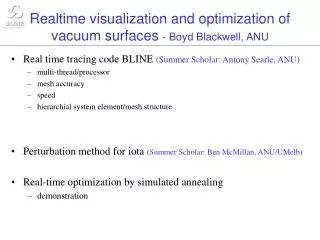
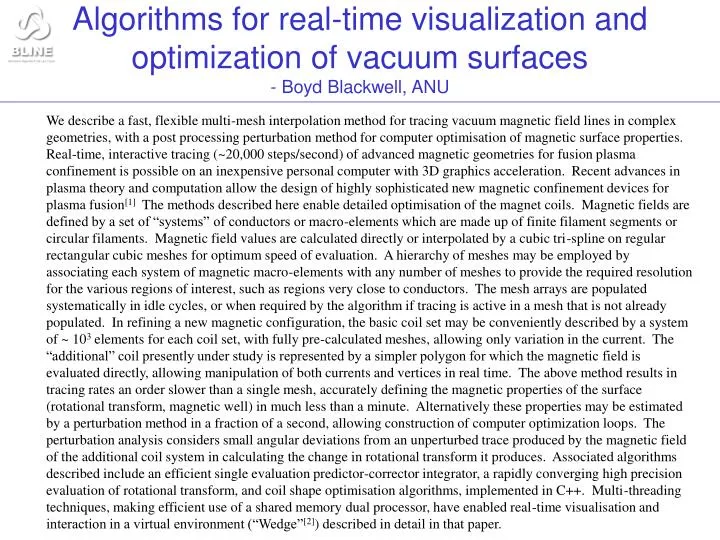
Algorithms for real-time visualization and optimization of vacuum surfaces - Boyd Blackwell, ANU We describe a fast, flexible multi-mesh interpolation method for tracing vacuum magnetic field lines in complex geometries, with a post processing perturbation method for computer optimisation of magnetic surface properties. Real-time, interactive tracing (~20,000 steps/second) of advanced magnetic geometries for fusion plasma confinement is possible on an inexpensive personal computer with 3D graphics acceleration. Recent advances in plasma theory and computation allow the design of highly sophisticated new magnetic confinement devices for plasma fusion[1] The methods described here enable detailed optimisation of the magnet coils. Magnetic fields are defined by a set of “systems” of conductors or macro-elements which are made up of finite filament segments or circular filaments. Magnetic field values are calculated directly or interpolated by a cubic tri-spline on regular rectangular cubic meshes for optimum speed of evaluation. A hierarchy of meshes may be employed by associating each system of magnetic macro-elements with any number of meshes to provide the required resolution for the various regions of interest, such as regions very close to conductors. The mesh arrays are populated systematically in idle cycles, or when required by the algorithm if tracing is active in a mesh that is not already populated. In refining a new magnetic configuration, the basic coil set may be conveniently described by a system of ~ 103 elements for each coil set, with fully pre-calculated meshes, allowing only variation in the current. The “additional” coil presently under study is represented by a simpler polygon for which the magnetic field is evaluated directly, allowing manipulation of both currents and vertices in real time. The above method results in tracing rates an order slower than a single mesh, accurately defining the magnetic properties of the surface (rotational transform, magnetic well) in much less than a minute. Alternatively these properties may be estimated by a perturbation method in a fraction of a second, allowing construction of computer optimization loops. The perturbation analysis considers small angular deviations from an unperturbed trace produced by the magnetic field of the additional coil system in calculating the change in rotational transform it produces. Associated algorithms described include an efficient single evaluation predictor-corrector integrator, a rapidly converging high precision evaluation of rotational transform, and coil shape optimisation algorithms, implemented in C++. Multi-threading techniques, making efficient use of a shared memory dual processor, have enabled real-time visualisation and interaction in a virtual environment (“Wedge”[2]) described in detail in that paper. Outline: • Real time tracing code BLINE (Summer Scholar: Antony Searle, ANU) • multi-thread/processor • mesh accuracy • speed • hierarchial system element/mesh structure • Perturbation method for iota (Summer Scholar: Ben McMillan, ANU/UMelb) • Real-time optimization by simulated annealing • example
Algorithms for real-time visualization and optimization of vacuum surfaces - Boyd Blackwell, ANU Outline: • Real time tracing code BLINE (Summer Scholar: Antony Searle, ANU) • multi-thread/processor • mesh accuracy • speed • hierarchial system element/mesh structure • Perturbation method for iota (Summer Scholar: Ben McMillan, ANU/UMelb) • Real-time optimization by simulated annealing • example
Minimal Confinement Geometries What is the simplest possible magnetic configuration that has the basic properties of, and similar parameters, to realistic plasma configurations? We require: • nested magnetic surfaces that enclose no conductors • the magnetic field can be evaluated very quickly • iota (twist per turn) ~ 1: aspect ratio low ~ 5-10 (“fat” torus) • highly 3D, so that codes and algorithms are tested thoroughly • represent by real conductors to ensure that Maxwell’s Eqns are satisfied • “triator” • only 4 simple elements (finite filaments) • iota ~ 0.6, bean shaped, (similar to Tom Todds?) • “single loop” toroidal helix: curiosity • slow evaluation
Mesh Interpolation H-1 heliac Pre-calculate magnetic field B on hierarchy of rectangular meshes using a cubic tri-spline interpolation method • mesh hierarchy(blue) underneath the hierarchy of magnetic macro-elements (“sub-systems”) • e.g. H-1 has 3 meshes for main field, but one coarse mesh for VF (Helmholtz) coils. Additionalsmall, finer grids can be placed in criticalareas that are heavily travelled e.g. near helical core • Splitting coils into subsystems allows quick configuration adjustment by varying currents (linear combination I1M1 + I2M2 + I3M3) • copy of mesh in neighborhood stored as array to fit into CPU cache • subarray of mesh representing the neighbourhood of a point would be spread over a large fraction of memory, and would not fit into the Level 2 (512K) cache on the Pentium II. • keep local copy (4x4x4) of mesh in neighbourhood of present position • only one face has to be updated - usually the next trace step is quite close • 3D array derivatives calculated on demand from B and stored only in local mesh • reduces the time penalty for the large mesh “get” method (the local copy is accessed as an array) • mesh filled on demand and/or in background • (see also Gourdon code, Zacharov’s code (Hermite polynomials)) centralcore Toroidal coils 3 meshes of 16×128×16 Helmholtz coils 1 mesh 64×64×32 3 meshes of 32×128×32 3x3 submeshes 32×128×32
Cubic Spline Mesh Convergence A magnetic field line is traced by direct and mesh-based calculations. The average and worst case difference of the mesh-based from the direct calculation are shown. Convergence is better than 5th order in x. Meshes of 10-50MByte are adequate even near edge to allow for regions of high gradient near conductors, the distance to the nearest conductor is recorded in each cell, and Bline automatically reverts to direct calculation if too close to a conductor. 5th order or better in x
Fast, Single Evaluation Predictor-Corrector The most popular integration methods for magnetic field line tracing are Runge-Kutta (4th order - used by most codes to start up, no previous points requ’d) 4 evals Predictor-Corrector (The HELIAC code uses 3rd order predictor, 4th order corrector 2 evals In magnetic field line tracing applications, the derivative evaluation step is time consuming, so it is desirable to minimize the number of derivative evaluations per step. The BLINE code uses a single evaluation predictor-corrector Predictor: (four step, fourth order Adams-Bashforth) xpred = xi-1 + h/24 (55ƒ(xi-1) - 59ƒ(xi-2) + 37ƒ(xi-3) - 9ƒ(xi-4)) (no new evaluations) Corrector: (four step, fifth order Adams-Moulton) xi = xi-1 + h/24 (9ƒ(xpred) + 19ƒ(xi-1) - 5ƒ(xi-2) + ƒ(xi-3)) (only one evaluation of B(r)) The resulting speed improvement is a factor of 1.55 (Fujitsu VP2200) - 2x
Fast, Single Evaluation Predictor-Corrector The most popular integration methods for magnetic field line tracing are Runge-Kutta (4th order - used by most codes to start up, no previous points requ’d) 4 evals Predictor-Corrector (The HELIAC code uses 3rd order predictor, 4th order corrector 2 evals In magnetic field line tracing applications, the derivative evaluation step is time consuming, so it is desirable to minimize the number of derivative evaluations per step. The BLINE code uses a single evaluation predictor-corrector Predictor: (four step, fourth order Adams-Bashforth) xpred = xi-1 + h/24 (55ƒ(xi-1) - 59ƒ(xi-2) + 37ƒ(xi-3) - 9ƒ(xi-4)) (no new evaluations) Corrector: (four step, fifth order Adams-Moulton) xi = xi-1 + h/24 (9ƒ(xpred) + 19ƒ(xi-1) - 5ƒ(xi-2) + ƒ(xi-3)) (only one evaluation of B(r)) The resulting speed improvement is a factor of 1.55 (Fujitsu VP2200) - 2x
Multi-processing Multi-threading is an efficient way to utilize a low cost, multi-processor shared memory machine • use windows threads (posix under linux) (Multiple Instruction Single Data) • needs semaphore system (e.g. no tracing while loading a new mesh) • multi-threaded code runs fine on single processor (some priority tuning useful on single processor) • initial scheme • tracing thread, display thread and mesh-filling threads • large caches on Intel machines favour each thread working in distant memory locations to avoid slowdown by cache overlap conflicts • multi-threading object oriented coding
Perturbation Calculation of iota B B0 • Find a nearby rational surface by iteration ~ middle order • say ~ 30 circuits • Store B and derivatives along this closed path • For each iteration of the perturbing winding locus, integrate x B/B0 whereB is the perturbing field and B0 the original field • (Alternatively integrate cpt of B in the surface, normalized to B0 and the puncture spacing at that point ~ Boozer )
Accuracy of perturbation / I • Check perturbation calculation of /I by direct calculation of in the initial and slightly perturbed configurations. • Ultra high accuracy (<1e-7) calculations of iota necessary to check /I when perturbation is small to avoid non-linearity • Direct iota measurement uses apodised least-squares fit, converges exponentially once significant Fourier cpts are captured. • Correction for area changecan be significant Perturbation result: 0.315 cf 0.304
Computer Optimization of transform Simulated annealing: • virtual temperature T • accept a new configuration even if slightly worse (up to T) • “heat” to explore new configurations • “cool” to “home in” on optimum • Annealing more tolerant of occasional anomalies in “goodness” function, e.g. local minima or discontinuities (resonances) • Speed is increased by • use of perturbation technique for calculating transform • incremental changes in conductor locus - only two elements change • 3 fold and up/down symmetry speed up by a factor of 6x. • Minimization by steepest descent less suitable - highly multi-variate - typically 30-1000 variables, similarity to travelling salesman problem.
Optimization of iota reproduces flexible heliac Given an existing coil set, what is the most efficient way to add rotational transform (twist-per-turn)? • existing conductor set is a “standard heliac” • Constraint: additional conductor lies anywhere inside a torus, periodicity N=3 • (actually end-point and middle point fixed in each period) • Seek maximum in transform/(length current) • Result is very close to the “flexible heliac” configuration proposed for transform and well control by Harris et al, 1985 The optimized winding is shown in pink, and exaggerated in thickness for clarity against the thinner basic (existing) conductor configuration. Comparison of the optimzed conductor (blue) with the “flexible heliac” toroidal helix. Differences are mainly due to incomplete annealing.
Optimum conductor outside plasma: R=R0 constraint “sawtooth coil” • Constrain conductor to lie on a cylinder, periodic (N=3) • Seek maximum transform near the axis of a heliac per unit (length current) • Base configuration is heliac • Reproduces approximate “sawtooth coil”
Conclusions and Future Work • Very useful for following particles out of machine (so far, not a drift calculation) • Very quick (50k/sec) configuration evaluation for varying current ratios in existing coil system (e.g. H-1 flexibility studies) • Fast evaluation (10k/sec) of new winding (“simple”) in arbitrarily complex existing configuration • Iota perturbation calculation works, and is fast. • Well perturbation calculation implemented, but not debugged • Possibly extend to island width as in Rieman & Boozer 1983 • optimization principle demonstrated • “standard results” recovered • real time operation possibility of human guidance during optimization Develop/find “Meta-Language” for description of symmetries and constraints