Download
1 / 56
560 likes | 944 Vues
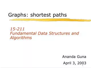
Graphs: shortest paths. 15-211 Fundamental Data Structures and Algorithms. Ananda Guna April 3, 2003. Announcements. Start working on Homework #5. Quiz #3 will be made available Friday 4/4 for 24 hours. . Recap. Vertices (aka nodes). Edges. Graphs — an overview. BOS.

E N D
Graphs: shortest paths 15-211 Fundamental Data Structures and Algorithms Ananda Guna April 3, 2003
Announcements • Start working on Homework #5. • Quiz #3 will be made available Friday 4/4 for 24 hours.
Vertices (aka nodes) Edges Graphs — an overview BOS 618 DTW SFO 2273 211 190 PIT 318 JFK 1987 344 2145 2462 LAX Weights (Undirected)
Definitions • Graph G = (V,E) • Set V of vertices (nodes) • Set E of edges • Elements of E are pair (v,w) where v,w V. • An edge (v,v) is a self-loop. (Usually assume no self-loops.) • Weighted graph • Elements of E are ((v,w),x) where x is a weight. • Directed graph (digraph) • The edge pairs are ordered • Undirected graph • The edge pairs are unordered • E is a symmetric relation • (v,w) E implies (w,v) E • In an undirected graph (v,w) and (w,v) are the same edge
Graph Questions • Is (x,y) an edge in the Graph? • Given x in V, does (x,x) in E? • Given x, y in V, what is the closest(cheapest) path from x to y (if any)? • What node v in V has the maximum(minimum) degree? • What is the largest connected sub-graph? • What is the complexity of algorithms for each of the above questions if • Graph is stored as an adjacency matrix? • Graph is stored as an adjacency list?
Graph Traversals • One of the fundamental operations in graphs. Find things such as • Count the total edges • Output the content in each vertex • Identify connected components • Before/during the tour - mark vertices • Visited • Not-visited • explored
Graph Traversals using.. • Queue - Store the vertices in a first-in, first out (FIFO) queue as follows. Put the starting node in a queue first. Dequeue the first element and add all its neighbors to the queue. Continue to explore the oldest unexplored vertices first. Thus the explorations radiate out slowly from the starting vertex. This describes a traversal technique known as breadth-first search. • Stack- Store vertices in a last-in, first-out (LIFO) stack. Explore vertices by going along a path, always visiting a new neighbor if one is available, and backing up only if all neighbors are discovered vertices. Thus our explorations quickly move away from start. This is called depth-first search.
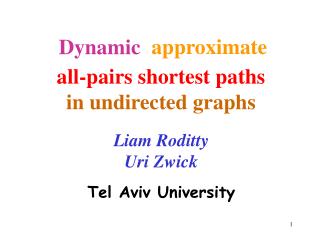
Airline routes 2704 BOS 867 1846 187 ORD 849 PVD SFO 740 144 JFK 802 1464 337 621 1258 184 BWI 1391 LAX DFW 1090 1235 946 1121 MIA 2342
Single-source shortest path • Suppose we live in Baltimore (BWI) and want the shortest path to San Francisco (SFO). • One way to solve this is to solve the single-source shortest path problem: • Find the shortest path from BWI to every city.
Single-source shortest path • While we may be interested only in BWI-to-SFO, there are no known algorithms that are asymptotically faster than solving the single-source problem for BWI-to-every-city.
Shortest paths • What do we mean by “shortest path”? • Minimize the number of layovers (i.e., fewest hops). • Unweighted shortest-path problem. • Minimize the total mileage (i.e., fewest frequent-flyer miles ;-). • Weighted shortest-path problem.
Many applications • Shortest paths model many useful real-world problems. • Minimization of latency in the Internet. • Minimization of cost in power delivery. • Job and resource scheduling. • Route planning.
Unweighted Single-Source Shortest Path Algorithm
Unweighted shortest path • In order to find the unweighted shortest path, we will augment vertices and edges so that: • vertices can be marked with an integer, giving the number of hops from the source node, and • edges can be marked as either exploredor unexplored. Initially, all edges are unexplored.
Unweighted shortest path • Algorithm: • Set i to 0 and mark source node v with 0. • Put source node v into a queue L0. • While Li is not empty: • Create new empty queue Li+1 • For each w in Lido: • For each unexplored edge (w,x) do: • mark (w,x) as explored • if x not marked, mark with i and enqueue x into Li+1 • Increment i.
Breadth-first search • This algorithm is a form of breadth-first search. • Performance: O(|V|+|E|). • Q: Use this algorithm to find the shortest route (in terms of number of hops) from BWI to SFO. • Q: What kind of structure is formed by the edges marked as explored?
Use of a queue • It is very common to use a queue to keep track of: • nodes to be visited next, or • nodes that we have already visited. • Typically, use of a queue leads to a breadth-first visit order. • Breadth-first visit order is “cautious” in the sense that it examines every path of length i before going on to paths of length i+1.
Weighted Single-Source Shortest Path Algorithm (Dijkstra’s Algorithm)
Weighted shortest path • Now suppose we want to minimize the total mileage. • Breadth-first search does not work! • Minimum number of hops does not mean minimum distance. • Consider, for example, BWI-to-DFW:
Three 2-hop routes to DFW 2704 BOS 867 1846 187 ORD 849 PVD SFO 740 144 JFK 802 1464 337 621 1258 184 BWI 1391 LAX DFW 1090 1235 946 1121 MIA 2342
A greedy algorithm • Assume that every city is infinitely far away. • I.e., every city is miles away from BWI (except BWI, which is 0 miles away). • Now perform something similar to breadth-first search, and optimistically guess that we have found the best path to each city as we encounter it. • If we later discover we are wrong and find a better path to a particular city, then update the distance to that city.
Intuition behind Dijkstra’s alg. • For our airline-mileage problem, we can start by guessing that every city is miles away. • Mark each city with this guess. • Find all cities one hop away from BWI, and check whether the mileage is less than what is currently marked for that city. • If so, then revise the guess. • Continue for 2 hops, 3 hops, etc.
Dijkstra’s algorithm • Algorithm initialization: • Label each node with the distance , except start node, which is labeled with distance 0. • D[v] is the distance label for v. • Put all nodes into a priority queue Q, using the distances as labels.
Dijkstra’s algorithm, cont’d • While Q is not empty do: • u = Q.removeMin • for each node z one hop away from u do: • if D[u] + miles(u,z) < D[z] then • D[z] = D[u] + miles(u,z) • change key of z in Q to D[z] • Note use of priority queue allows “finished” nodes to be found quickly (in O(log N) time).
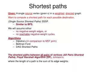
Shortest mileage from BWI 2704 BOS 867 1846 187 ORD 849 PVD SFO 740 144 JFK 802 1464 337 621 1258 184 BWI 0 1391 LAX DFW 1090 1235 946 1121 MIA 2342
Shortest mileage from BWI 2704 BOS 867 1846 187 ORD 621 849 PVD SFO 740 144 JFK 184 802 1464 337 621 1258 184 BWI 0 1391 LAX DFW 1090 1235 946 1121 MIA 946 2342
Shortest mileage from BWI 2704 BOS 371 867 1846 187 ORD 621 849 PVD 328 SFO 740 144 JFK 184 802 1464 337 621 1258 184 BWI 0 1391 LAX DFW 1575 1090 1235 946 1121 MIA 946 2342
Shortest mileage from BWI 2704 BOS 371 867 1846 187 ORD 621 849 PVD 328 SFO 740 144 JFK 184 802 1464 337 621 1258 184 BWI 0 1391 LAX DFW 1575 1090 1235 946 1121 MIA 946 2342
Shortest mileage from BWI 2704 BOS 371 867 1846 187 ORD 621 849 PVD 328 SFO 3075 740 144 JFK 184 802 1464 337 621 1258 184 BWI 0 1391 LAX DFW 1575 1090 1235 946 1121 MIA 946 2342
Shortest mileage from BWI 2704 BOS 371 867 1846 187 ORD 621 849 PVD 328 SFO 2467 740 144 JFK 184 802 1464 337 621 1258 184 BWI 0 1391 LAX DFW 1423 1090 1235 946 1121 MIA 946 2342
Shortest mileage from BWI 2704 BOS 371 867 1846 187 ORD 621 849 PVD 328 SFO 2467 740 144 JFK 184 802 1464 337 621 1258 184 BWI 0 1391 LAX 3288 DFW 1423 1090 1235 946 1121 MIA 946 2342
Shortest mileage from BWI 2704 BOS 371 867 1846 187 ORD 621 849 PVD 328 SFO 2467 740 144 JFK 184 802 1464 337 621 1258 184 BWI 0 1391 LAX 2658 DFW 1423 1090 1235 946 1121 MIA 946 2342
Shortest mileage from BWI 2704 BOS 371 867 1846 187 ORD 621 849 PVD 328 SFO 2467 740 144 JFK 184 802 1464 337 621 1258 184 BWI 0 1391 LAX 2658 DFW 1423 1090 1235 946 1121 MIA 946 2342
Shortest mileage from BWI 2704 BOS 371 867 1846 187 ORD 621 849 PVD 328 SFO 2467 740 144 JFK 184 802 1464 337 621 1258 184 BWI 0 1391 LAX 2658 DFW 1423 1090 1235 946 1121 MIA 946 2342
Shortest mileage from BWI 2704 BOS 371 867 1846 187 ORD 621 849 PVD 328 SFO 2467 740 144 JFK 184 802 1464 337 621 1258 184 BWI 0 1391 LAX 2658 DFW 1423 1090 1235 946 1121 MIA 946 2342
Dijkstra’s algorithm, recap • While Q is not empty do: • u = Q.removeMin • for each node z one hop away from u do: • if D[u] + miles(u,z) < D[z] then • D[z] = D[u] + miles(u,z) • change key of z in Q to D[z]
Quiz break • Would it be better to use an adjacency list or an adjacency matrix for Dijkstra’s algorithm? • What is the running time of Dijkstra’s algorithm, in terms of |V| and |E|?
Complexity of Dijkstra • Adjacency matrix version Dijkstra finds shortest path from one vertex to all others in O(|V|2) time • If |E| is small compared to |V|2, use a priority queue to organize the vertices in V-S, where V is the set of all vertices and S is the set that has already been explored • So total of |E| updates each at a cost of O(log |V|) • So total time is O(|E| log|V|)
The All Pairs Shortest Path Algorithm (Floyd’s Algorithm)
Finding all pairs shortest paths • Assume G=(V,E) is a graph such that c[v,w] 0, where C is the matrix of edge costs. • Find for each pair (v,w), the shortest path from v to w. That is, find the matrix of shortest paths • Certainly this is generalization of Dijkstra’s. • Note: For later discussions assume |V| = n and |E| = m
Floyd’s Algorithm • A[i][j] = C(i,j) if there is an edge (i,j) • A[i][j] = infinity(inf) if there is no edge (i,j) Graph “adjacency” matrix A is the shortest path matrix that uses 1 or fewer edges
Floyd ctd.. • To find shortest paths that uses 2 or fewer edges find A2, where multiplication defined as min of sums instead sum of products • That is (A2)ij = min{ Aik + Akj | k =1..n} • This operation is O(n3) • Using A2 you can find A4 and then A8 and so on • Therefore to find An we need log n operations • Therefore this algorithm is O(log n* n3) • We will consider another algorithm next
Floyd-Warshall Algorithm • This algorithm uses nxn matrix A to compute the lengths of the shortest paths using a dynamic programming technique. • Let A[i,j] = c[i,j] for all i,j & ij • If (i,j) is not an edge, set A[i,j]=infinity and A[i,i]=0 • Ak[i,j] = min (Ak-1[i,j] , Ak-1[i,k]+ Ak-1[k,j])
Example – Floyd’s Algorithm Find the all pairs shortest path matrix 8 2 1 2 3 3 5 • Ak[i,j] = min (Ak-1[i,j] , Ak-1[i,k]+ Ak-1[k,j])
Floyd-Warshall Implementation • initialize A[i,j] = C[i,j] • initialize all A[i,i] = 0 • for k from 1 to n for i from 1 to n for j from 1 to n if (A[i,j] > A[i,k]+A[k,j]) A[i,j] = A[i,k]+A[k,j]; • The complexity of this algorithm is O(n3)
Negative Weighted Single-Source Shortest Path Algorithm (Bellman-Ford Algorithm)
Bellman-Ford Algorithm Definition: An efficient algorithm to find the shortest paths from a single sourcevertex to all other vertices in a weighted, directed graph. Weights may be negative. The algorithm initializes the distance to the source vertex to 0 and all other vertices to . It then does V-1 passes (V is the number of vertices) over all edges relaxing, or updating, the distance to the destination of each edge. Finally it checks each edge again to detect negative weight cycles, in which case it returns false. The time complexity is O(VE), where E is the number of edges. Source: NIST
Bellman-Ford Shortest Paths • We want to compute the shortest path from the start to every node in the graph. As usual with DP, let's first just worry about finding the LENGTH of the shortest path. We can later worry about actually outputting the path. • To apply the DP approach, we need to break the problem down into sub-problems. We will do that by imagining that we want the shortest path out of all those that use i or fewer edges. We'll start with i=0, then use this to compute for i=1, 2, 3, ....