Download
1 / 33
480 likes | 898 Vues
Chapter 1 Introduction and Background to Quantum Mechanics. The Need for Quantum Mechanics in Chemistry. Without Quantum Mechanics, how would you explain:. • Periodic trends in properties of the elements. • Structure of compounds

E N D
Chapter 1 Introduction and Background to Quantum Mechanics
The Need for Quantum Mechanics in Chemistry Without Quantum Mechanics, how would you explain: • Periodic trends in properties of the elements • Structure of compounds e.g. Tetrahedral carbon in ethane, planar ethylene, etc. • Bond lengths/strengths • Discrete spectral lines (IR, NMR, Atomic Absorption, etc.) • Electron Microscopy Without Quantum Mechanics, chemistry would be a purely empirical science. PLUS:In recent years, a rapidly increasing percentage of experimental chemists are performing quantum mechanical calculations as an essential complement to interpreting their experimental results.
Outline • Problems in Classical Physics • The “Old” Quantum Mechanics (Bohr Theory) • Wave Properties of Particles • Heisenberg Uncertainty Principle • Mathematical Preliminaries • Concepts in Quantum Mechanics There is nothing new to be discovered in Physics now. All that remains is more and more precise measurement. Lord Kelvin (Sir William Thompson), ca 1900
Heated Metal Low Temperature: Red Hot Intermediate Temperature: White Hot High Temperature: Blue Hot Intensity Blackbody Radiation
Rayleigh-Jeans (Classical Physics) Assumed that electrons in metal oscillate about their equilibrium positions at arbitrary frequency (energy). Emit light at oscillation frequency. The Ultraviolet Catastrophe: Intensity
Max Planck (1900) Arbitrarily assumed that the energy levels of the oscillating electrons are quantized, and the energy levels are proportional to : = h(n) n = 1, 2, 3,... h = empirical constant He derived the expression: Expression matches experimental data perfectly for Intensity h = 6.626x10⁻³⁴ J•s [Planck’s Constant]
Kinetic Energy of ejected electrons can be measured by determining the magnitude of the “stopping potential” (VS) required to stop current. - VS + Observations A Low frequency (red) light: < o - No ejected electrons (no current) High frequency (blue) light: > o - K.E. of ejected electrons K.E. o The Photoelectric Effect
Photons Einstein (1903) proposed that light energy is quantized into “packets” called photons. Slope = h Eph = h Explanation of Photoelectric Effect Eph = h = + K.E. is the metal’s “work function”: the energy required to eject an electron from the surface K.E. = h - = h - ho Predicts that the slope of the graph of K.E. vs. is h (Planck’s Constant) o = / h K.E. in agreement with experiment !! o
Equations Relating Properties of Light Wavelength/ Frequency: Wavenumber: Units: cm-1 c must be in cm/s Energy: You should know these relations between the properties of light. They will come up often throughout the course.
Sample Heat When a sample of atoms is heated up, the excited electrons emit radiation as they return to the ground state. The emissions are at discrete frequencies, rather than a continuum of frequencies, as predicted by the Rutherford planetary model of the atom. Atomic Emission Spectra
Hydrogen Atom Emission Lines UV Region: (Lyman Series) n = 2, 3, 4 ... Visible Region: (Balmer Series) n = 3, 4, 5, ... Infrared Region: (Paschen Series) n = 4, 5, 6 ... General Form (Johannes Rydberg) n1 = 1, 2, 3 ... n2 > n1 RH = 108,680 cm-1
Outline • Problems in Classical Physics • The “Old” Quantum Mechanics (Bohr Theory) • Wave Properties of Particles • Heisenberg Uncertainty Principle • Mathematical Preliminaries • Concepts in Quantum Mechanics
Niels Bohr (1913) Assumed that electron in hydrogen-like atom moved in circular orbit, with the centripetal force (mv2/r) equal to the Coulombic attraction between the electron (with charge e) and nucleus (with charge Ze). e r Ze (Dirac’s Constant) He then arbitrarily assumed that the “angular momentum” is quantized. n = 1, 2, 3,... The “Old” Quantum Theory Why?? Because it worked.
It can be shown = 0.529 Å (Bohr Radius) n = 1, 2, 3,...
nU EU nL EL Lyman Series: nL = 1 Balmer Series: nL = 2 Paschen Series: nL = 3
nU EU nL EL Close to RH = 108,680 cm-1 Get perfect agreement if replace electron mass (m) by reduced mass () of proton-electron pair.
The Bohr Theory of the atom (“Old” Quantum Mechanics) works perfectly for H (as well as He+, Li2+, etc.). And it’s so much EASIER than the Schrödinger Equation. The only problem with the Bohr Theory is that it fails as soon as you try to use it on an atom as “complex” as helium.
Outline • Problems in Classical Physics • The “Old” Quantum Mechanics (Bohr Theory) • Wave Properties of Particles • Heisenberg Uncertainty Principle • Mathematical Preliminaries • Concepts in Quantum Mechanics
and Wave Properties of Particles The de Broglie Wavelength Louis de Broglie (1923): If waves have particle-like properties (photons, then particles should have wave-like properties. Photon wavelength-momentum relation de Broglie wavelength of a particle
What is the de Broglie wavelength of a 1 gram marble traveling at 10 cm/s h=6.63x10⁻³⁴ J-s What is the de Broglie wavelength of an electron traveling at 0.1 c (c=speed of light)? c = 3.00x10⁸ m/s me = 9.1x10⁻³¹ kg = 6.6x10⁻³⁰ m = 6.6x10⁻²⁰Å (insignificant) = 2.4x10⁻¹¹ m = 0.24 Å (on the order of atomic dimensions)
n = 1, 2, 3,... (Dirac’s Constant) Reinterpretation of Bohr’s Quantization of Angular Momentum The circumference of a Bohr orbit must be a whole number of de Broglie “standing waves”.
Outline • Problems in Classical Physics • The “Old” Quantum Mechanics (Bohr Theory) • Wave Properties of Particles • Heisenberg Uncertainty Principle • Mathematical Preliminaries • Concepts in Quantum Mechanics
Werner Heisenberg: 1925 It is not possible to determine both the position (x) and momentum (p) of a particle precisely at the same time. p = Uncertainty in momentum x = Uncertainty in position Heisenberg Uncertainty Principle There are a number of pseudo-derivations of this principle in various texts, based upon the wave property of a particle. We will not give one of these derivations, but will provide examples of the uncertainty principle at various times in the course.
Calculate the uncertainty in the position of a 5 Oz (0.14 kg) baseball traveling at 90 mi/hr (40 m/s), assuming that the velocity can be measured to a precision of 10-6 percent. h = 6.63x10⁻³⁴ J-s ħ = 1.05x10⁻³⁴ J-s1 x = 9.4x10⁻²⁸ m Calculate the uncertainty in the momentum (and velocity) of an electron (me=9.11x10⁻³¹ kg) in an atom with an uncertainty in position, x = 0.5 Å = 5x10-11 m. p = 1.05x10⁻²⁴ kgm/s v = 1.15x10⁶ m/s (=2.6x10⁶ mi/hr)
Outline • Problems in Classical Physics • The “Old” Quantum Mechanics (Bohr Theory) • Wave Properties of Particles • Heisenberg Uncertainty Principle • Mathematical Preliminaries • Concepts in Quantum Mechanics
y axis cos() = x sin() = y 1 y x axis x Math Preliminary: Trigonometry and the Unit Circle sin(0o) = 0 cos(180o) = -1 sin(90o) = 1 cos(270o) = 0 From the unit circle, it’s easy to see that: cos(-) = cos() sin(-) = -sin()
Imag axis Euler Relations R y Real axis x or where Complex Plane or Math Preliminary: Complex Numbers Complex number (z) Complex conjugate (z*)
Imag axis R y Real axis x or where Complex Plane Math Preliminary: Complex Numbers Magnitude of a Complex Number or
Outline • Problems in Classical Physics • The “Old” Quantum Mechanics (Bohr Theory) • Wave Properties of Particles • Heisenberg Uncertainty Principle • Mathematical Preliminaries • Concepts in Quantum Mechanics
Concepts in Quantum Mechanics Erwin Schrödinger (1926): If, as proposed by de Broglie, particles display wave-like properties, then they should satisfy a wave equation similar to classical waves. He proposed the following equation. One-Dimensional Time Dependent Schrödinger Equation is the wavefunction ||2 = * is the probability of finding the particle between x and x + dx m = mass of particle V(x,t) is the potential energy
- + V(x,t) = const = 0 where and Classical Traveling Wave For a particle: Unsatisfactory because The probability of finding the particle at any position (i.e. any value of x) should be the same is satisfactory Note that: Wavefunction for a free particle
where and on board on board “Derivation” of Schrödinger Eqn. for Free Particle Schrödinger Eqn. for V(x,t) = 0
Note: We cannot actually derive Quantum Mechanics or the Schrödinger Equation. In the last slide, we gave a rationalization of how, if a particle behaves like a wave and is given by the de Broglie relation, then the wavefunction, , satisfies the wave equation proposed by Erwin Schrödinger. Quantum Mechanics is not “provable”, but is built upon a series of postulates, which will be discussed in the next chapter. The validity of the postulates is based upon the fact that Quantum Mechanics WORKS. It correctly predicts the properties of electrons, atoms and other microscopic particles.