Download
1 / 34
340 likes | 469 Vues
2. Analysis of frequency counts with Chi square. Dr David Field. Summary. Categorical data Frequency counts One variable chi-square testing the null hypothesis that frequencies in the sample are equally divided among the catgegories varying the null hypothesis Two variable chi-square

E N D
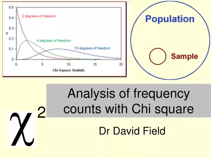
2 Analysis of frequency counts with Chi square Dr David Field
Summary • Categorical data • Frequency counts • One variable chi-square • testing the null hypothesis that frequencies in the sample are equally divided among the catgegories • varying the null hypothesis • Two variable chi-square • testing the null hypothesis that status on one categorical variable is independent from status on another categorical variable • Limitations and assumptions of chi-square • Andy Field chapter 18 covers chi-square • There is also a guide online at • http://davidmlane.com/hyperstat/ • Chi-square is topic 16 in the list
Categorical data 18.2 • Each participant is a member of a single category, and the categories cannot be meaningfully placed in order • e.g., nationality = French, German, Italian • Sometimes chi-square is used with ordered categories, e.g. age bands • To perform statistical tests with categorical data each participant must be a member of only one category • Category membership must be mutually exclusive • You can’t be a smoker and a non-smoker • This allows frequency counts in each category to be calculated
2 Chi square • If you can express the data as frequency counts in several categories, then chi square can be used to test for differences between the categories • You will also see chi square written as a Greek letter accompanied by the mathematical symbol indicating that a number should be squared
Chi square with a single categorical variable • Suppose we are interested in which drink is most popular • We ask a sample of 100 people if they prefer to drink coffee, tea, or water • each respondent is only allowed to select one answer • this is important: if each person can have membership of more than one category you can’t use Chi square • By default, the null hypothesis for chi-square is that each of the categories is equally frequent in the underlying population • it is possible to modify this (see later)
One variable chi-square example • Let’s say that the preferences expressed by the sample of 100 people result in the following observed frequency counts: • tea 39 • coffee 30 • Water 31 • SUM 100 • The null hypothesis assumes that each category is equally frequent, and thus provides a model that the data can be used to test • Based on the null hypothesis, the expected frequency counts would 100 / 3 = 33.3 per category • The Chi square statistic works out the probability that the observed frequencies could be obtained by random sampling from a population where the null hyp is true
Converting Chi square to a p value • SPSS will do this for you • Chi square has degrees of freedom equal to the number of categories minus 1 • 2 in the example this is because if you knew the frequencies of preference for tea and coffee and the sample size, the frequency of preference for water would not be free to vary • “The chi square value of 1.47, df = 2 had an associated p value of 0.48, so the null hypothesis that preferences for drinking tea, coffee and water in the population are equal cannot be rejected.”
One variable chi square with unequal expected frequencies • By default, the expected frequencies are just the sample size divided equally among the number of categories. • But, sometimes this is inappropriate • For example, we know that the % of the population of the UK that smokes is less than 50% • Let’s assume for purposes of illustration that 25% of the UK population are smokers • We might hypothesise that the smoking rate is higher in Glasgow than the UK average rate • The null hypothesis is that it is the same
One variable chi square with unequal expected frequencies • We ask 200 adults in Glasgow if they smoke. • 80 say yes • 120 say no • We know that the UK average rate is 25%, and 80 is rather more than 25% of 200 • Chi square can be used to assess the probability of the above frequencies being obtained by random sampling if the real smoking rate in Glasgow was actually 25%
One variable chi-square example with unequal expected frequencies
One variable chi square with unequal expected frequencies • “80 of the sample of 200 people from Glasgow classified themselves as smokers. This resulted in a chi square value of 24.0, df = 1 with an associated p value of < 0.001, so the null hypothesis that smoking rates in Glasgow are equal to the UK average of 25% can be rejected.”
18.3 Chi square with two variables • Usually, it is more interesting to use Chi square to ask about the relationship between 2 categorical variables. • For example, what is the relationship between gender and smoking? • gender can be male or female • smoking can be smoker or non-smoker • If you have smoking data from just men, you can only use chi-square to ask if the proportion of smokers and non-smokers is different • If you have smoking data from men and women you can use chi-square to ask if the proportion of men who smoke differs from the proportion of women who smoke
What 2*2 chi square does not do • It is important to realise that in the 2*2 chi square, having a big imbalance between the number of men and the number of women will not increase the value of the chi-square statistic • Also, having a big imbalance between the number of smokers and non-smokers will not increase the value of the chi-square statistic • This contrasts with the one variable chi-square, where an imbalance in the numbers of men vs women, or smokers vs. non-smokers does increase the value of chi-square. • The value of chi-square for two variables is high if smoking frequency is contingent on gender, and low if smoking frequency is independent of gender
The key to understanding 2*2 chi square is how the expected frequencies are calculated • The expected frequencies provide the null hypothesis, or null model, that the chi square statistic tests • If there are 200 participants, the simplest null model would be to expect 50 female smokers, 50 male smokers, 50 female non smokers, and 50 male non smokers • but we already know that it is implausible to expect an equal split of smokers and non-smokers • the expected frequencies will have to allow for the imbalance of smokers vs non smokers and a possible imbalance of men vs women in the sample • A sample with 20 male smokers, 10 female smokers, 80 male non-smokers and 40 female non-smokers has an imbalance of gender and smoking status, but smoking status does not depend on gender and there is no deviation from the null model
Calculating the expected frequencies • The key step in the calculation of chi-square is to estimate the frequency counts that would occur in each cell if the null hypothesis that the row frequencies and column frequencies do not depend upon each other were true • To calculate the expected frequency of the male smokers cell, we first need to calculate the proportion of participants that are male, without considering if they smoke or not • This proportion is 42 males out of 159 (the total number of participants) • 42 / 159 = 0.26
Calculating the expected frequencies • If the null hyp is true, and the proportion of female smokers and male smokers is equal, then the proportion of the smokers in the sample that are male should be equal to the overall proportion of the sample that is male • Total number of smokers in sample (44) * proportion of sample that is male (0.26) • 44 * 0.26 = 11.62
Calculating the value of chi square • Each cell in the contingency table makes a contribution to the total chi-square • For each cell you calculate • (Observed – Expected) and square it • You then divide by the Expected • Do this for each cell individually and add up the results
Calculating chi square (13-11.62)2 = 1.90 1.90 / 11.62 = 0.16
Converting chi-square to a p value • The degrees of freedom for a two way Chi square depends upon the number of categories in the contingency table • (num columns -1) * (num rows -1) • SPSS will calculate the DF and p value for you • “The chi square value of 0.31, df = 1 had an associated p value of 0.58, so the null hypothesis that the proportion of men and women that smoke is equal cannot be rejected.” • Also see 18.5.7
Larger contingency tables • You can perform chi-square on larger contingency tables • For example, we might be interested in whether the proportion of smokers vs. non smokers differs according to age, where age is a 3 level categorical variable • 20-29 years old • 30-39 years old • 40-49 years old • This results in a 2 * 3 contingency table • However, there is some uncertainty as to what a significant chi-square means in this case
Partitioning chi-square • A statistically significant 2 * 3 chi-square might have occurred for one of these 3 reasons • The proportion of 20-29 year olds who smoke differs from the proportion of 30-39 year olds that smoke • The proportion of 20-29 year olds that smoke differs from the proportion of 40-49 year olds that smoke • The proportion of 30-39 year olds that smoke differs from the proportion of 40-49 year olds that smoke • Or all 3 of the above might be true • Or 2 of the above might be true • As a researcher, you will want to distinguish between these possibilities
Partitioning chi-square • The solution is to break the 2 * 3 contingency table into smaller 2 * 2 contingency tables to test each of the comparisons in the list • The proportion of 20-29 year olds who smoke differs from the proportion of 30-39 year olds that smoke • The proportion of 20-29 year olds that smoke differs from the proportion of 40-49 year olds that smoke • The proportion of 30-39 year olds that smoke differs from the proportion of 40-49 year olds that smoke • Run 3 separate 2 * 2 chi-square tests
Partitioning chi-square • However, running 3 tests results in 3 chances of a type 1 error occurring • To maintain the probability of a type 1 error at the conventional level of 5% you divide the alpha level by the number of chi-square tests you run • Effectively, you share the 5% risk of rejecting the null hypothesis due to sampling error equally among the tests you perform • For a single chi-square, it is significant if SPSS reports that p is less than 0.05 • For two chi-square tests, they are significant at the 0.05 level individually if SPSS reports that p is less than 0.025 • For three chi-square tests, they are significant at the 0.05 level individually if SPSS reports that p is less than 0.0166
Warnings about chi-square • The expected frequency count in any cell must not be less than 5 • If this occurs then chi-square is not reliable • If the contingency table is 2 * 2 or 2 * 3 you can use the Fisher exact probability test instead • SPSS will report this • For bigger contingency tables the only solution is to “collapse” across categories, but only where this is meaningful • If you began with age categories 0-4, 5-10, 11-15, 16-20 you could collapse to 0-10 and 11-20, which would increase the expected frequencies in each cell • Finally, remember that the total of frequencies is equal to the number of participants you have • each person must only be a member of one cell in the table