Download
1 / 57
580 likes | 760 Vues
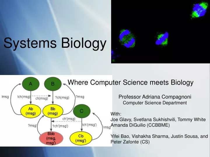
Systems Biology. Where Computer Science meets Biology. Professor Adriana Compagnoni Computer Science Department. With: Joe Glavy, Svetlana Sukhishvili, Tommy White Amanda DiGuilio (CCBBME) Yifei Bao, Vishakha Sharma, Justin Sousa, and Peter Zafonte (CS). Overview. The Virtual Lab

E N D
Systems Biology Where Computer Science meets Biology Professor Adriana Compagnoni Computer Science Department With: Joe Glavy, Svetlana Sukhishvili, Tommy White Amanda DiGuilio (CCBBME) Yifei Bao, Vishakha Sharma, Justin Sousa, and Peter Zafonte (CS)
Overview • The Virtual Lab • Modeling HER2 • Modeling Bio-films • Experimenting with 5 different modeling techniques • Modeling the G-protein Cycle • Incorporating Space
HER2 – Signaling Pathways • HER signaling is initiated when two receptor molecules join together in a process called dimerization, which occurs in response to the presence of a growth factor molecule (ligand). • Dimerization of different members of ErbB family, lead to activation of different kinase mediated intracellular signaling cascades, like • PI3 K/AKT pathway • MAPK pathway • JAK/STAT pathway
Differential HER2 concentrations a. 100 HER2 are initialized a. 30 HER2 are initialized
Inhibition of Raf activation(activation rate is changed from 27.0 to 1.0E-4 ) Pathways Crosstalk
3.2 μm 3.2 μm Hydrogen-bonded multilayer destruction Changing pH fast release of capsule cargo
Computational Modeling For The G-protein Cycle • Using 5 different modeling techniques: • Differential equations • Stochastic Pi-calculus • Stochastic Petri-Nets • Kappa • Bio-Pepa 12
G-Protein Couple Receptors(GPCRs) • G-protein couple receptors (GPCRs) sense molecules outside the cell and activate inside signal transduction pathways. • An estimated 50% of the current pharmaceuticals target GPCRs. 13
Activation cycle of G-proteins by G-protein-coupled receptors 2 1 3 5 4 14
The law of mass action • The law of mass action is a mathematical model that prescribes the evolution of a chemical system in terms of changes of concentrations of the chemical species over time. • In its simplest form, it says that a reaction X+Yk Z has a rate k[X][Y]: the rate is proportional to the concentration of one species ([X]) times the concentration of the other species ([Y]) by the base rate k. 16
Process AlgebrasAn alternative ot ODEs Formal languages originally designed to model complex reactive computer systems. Because of the similarities between reactive computer systems and biological systems, process algebra have recently been used to model biological systems. 18
Process Algebras Typically two halves of a communication: Sending and Receiving. !ch(msg) : to send message msg on channel ch. ?ch(msg) : to receive a message msg on channel ch. 19
Process Algebras A = new msg !ch (msg); Ab(msg) B = ?ch(msg); Bb (msg) Ab(msg) = !msg(); A Bb(msg) = ?msg(); B A and B bind A and B dissociate 20
Stochastic Pi-Calculus The stochastic pi-calculus is a process algebra where stochastic rates are imposed on processes, allowing a more accurate description of biological processes. SPiM (stochastic pi machine) is an implementation of the stochastic pi-calculus that can be used to run in-silico simulations that display the change over time in the populations of the different species of the system being modeled.
Step 1 to Step 2 2 1 !bindb Gd G ?bindb Gbg Gd represents alpha Gbg represents the beta-gamma complex 22
SPiM directive plot RL(); abrD(); aT()
Petri Nets Modeling The basic Petri Net is a directed bipartite graph with two kinds of nodes which are either places or transitions and directed arcs which connect nodes. In modeling biological processes, place nodes represent molecular species and transition nodes represent reactions. We use Cell Illustrator to develop our model of the G-protein cycle (www.cellillustrator.com). 30
Petri Nets Modeling NJPLS2010@Stevens
Petri Nets Modeling NJPLS2010@Stevens
Petri Nets Modeling NJPLS2010@Stevens
Petri Nets Modeling NJPLS2010@Stevens
Petri Nets Modeling NJPLS2010@Stevens
Petri Nets Modeling NJPLS2010@Stevens
Kappa Language Modeling Kappa is a formal language for defining agents (typically meant to represent proteins) as sets of sites that constitute abstract resources for interaction. It is used to express rules of interactions between proteins characterized by discrete modification and binding states. The Kappa language modeling platform is Cellucidate.
Kappa Language Modeling R and L are agent names, r is the binding site of R, l is the binding site of L, and 3.32e-09 is the reaction rate. In R(r!1) and L(l!1), 1 is the index of the link that binds R and L at their binding sites. R + L -> RL R(r), L(l)->R(r!1), L(l!1) @ 3.32e-09
Bio-PEPA Modeling Bio-PEPA is a process algebra for the modeling and the analysis of biochemical networks. It is a modification of PEPA to deal with some features of biological models, such as stoichiometry and the use of generic kinetic laws.
High Level Notations (motivation) Both ODEs and Petri Nets correspond closely to chemical reactions, and for the average biologist, they are relatively easy to understand. Cellucidate provides a friendly user interface for Kappa that abstracts away from its syntax. SPiM still needs encoding in the stochastic Pi-calculus.
High Level Notation (motivation) In order to hide Pi-calculus communication primitives and enable modeling using only terminology directly obtained from biological processes, we develop a high level notation that can be systematically translated into SPiM programs.
G-protein Cycle 2 bind bind 1 3 activate and dissociate hydrolyze 5 4 dissociate 48
Step 1 to Step 2 2 1 bind(Gd, Gbg, G, 1.0) 49
High Level Notation bind(Gd, Gbg, G, 1.0); bind(R, L, RL, 3.32e-6); activateAnddissociate(G, RL, Ga, Gbg, 1.0e-5); dissociate(RL, R, L, 0.01); hydrolyze(Ga, Gd, 0.11); degrade(R, 4e-4); degrade(RL, 4e-3)