Download
1 / 14
160 likes | 470 Vues
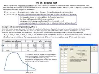
Chi-Squared Test Statistic. Summarize closeness of f o and f e by where sum is taken over all cells in the table. When H 0 is true, the sampling distribution of this statistic (for large n ) is approximately the chi-squared probability distribution . Problem: 8.7 and 8.9.

E N D
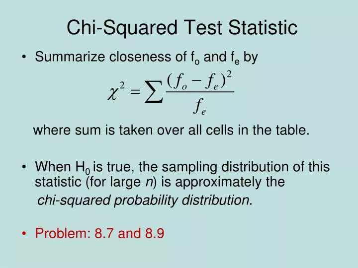
Chi-Squared Test Statistic • Summarize closeness of foand fe by where sum is taken over all cells in the table. • When H0 is true, the sampling distribution of this statistic (for large n) is approximately the chi-squared probability distribution. • Problem: 8.7 and 8.9
Limitations of the chi-squared test • The chi-squared test merely analyzes the extent of evidence that there is an association. • Does not tell us the nature of the association (standardized residuals are useful for this) • Does not tell us the strength of association. • e.g., a large chi-squared test statistic and small P-value indicates strong evidence of association but not necessarily a strong association. (Recall statistical significance not the same as practical significance.)
Residuals: Detecting Patterns of Association • Large chi-squared implies strong evidence of association but does not tell us about nature of association. We can investigate this by finding the residual in each cell of the contingency table. • Residual = fo-feis positive (negative) when there are more (fewer) observations in cell than null hypothesis of independence predicts. • Standardized residualz = (fo-fe)/se, where se denotes se of fo-fe.. This measures number of standard errors that (fo-fe) falls from value of 0 expected when H0 true.
The se value is found using • So, the standardized residual z = (fo-fe)/se equals • Example: For cell with fo= 272, fe= 189.6, row prop. = 615/2955 = 0.208, column prop. = 911/2955 = 0.308, and standardized residual • Number of people very happy and with above average family income is 8 standard errors higher than we’d expect if happiness were independent of income.
SPSS Output • Standardized (=adjusted) residualz = (fo-fe)/se
Likewise, we see more people in the (below average, not too happy) cell than expected, and fewer in (below average, very happy) and (above average, not too happy) cells than expected. • In cells having |standardized residual| > about 3, departure from independence is noteworthy (probably not just due to “chance” variability). • Standardized residuals can be found using some software (called adjusted residuals in SPSS). • Problem: 8.14
Measures of Association • Chi-squared test answers “Is there an association?” • Standardized residuals answer “How do data differ from what independence predicts?” • Now we ask “How strong is the association?” and analyze by using a measure of the effect size
The “odds” For two outcomes (“success”, “failure”) for a group, Odds = P(success)/P(failure) = P(success) / (1 - P(success)) e.g., if P(success) = 0.80, P(failure) = 0.20, the odds = 0.80/0.20 = 4.0 if P(success) = 0.20, P(failure) = 0.80, the odds = 0.20/0.80 = ¼ = 0.25 Probability of success can be obtained from odds by Probability = odds/(odds + 1) e.g., odds = 4.0 has probability = 4/(4+1) = 4/5 = 0.80
The odds ratio • For 2 groups summarized in a 2x2 contingency table, odds ratio = (odds in row 1)/(odds in row 2) Example: Survey of senior high school students Alcohol use Cigarette use Yes No Yes 1449 46 No 500 281 2 = 451.4, df= 1 (P-value = 0.00000…..) Standardized residuals all equal +21.2 or – 21.2.
For those who have smoked, the odds of having used alcohol are 1449/46 = 31.50. • For those who have not smoked, the odds of having used alcohol are 500/281 = 1.78 • The odds ratio = 31.5/1.78 = 17.7 • The estimated odds that smokers have used alcohol are 17.7 times the estimated odds that non-smokers have used alcohol.
Properties of the odds ratio The odds ratio … • Is non-negative • Is 1 when there is “no effect” • Falls farther from 1 or closer to 0 the stronger the association. • Takes same value regardless of choice of response variable. • Can be computed as a cross-product ratio. Example: Alcohol use Cigarette use Yes No Total Yes 1449 46 1495 No 500 281 781 odds ratio = (1449)(281)/(46)(500) = 17.7 • Problem: 8.20b • Se mere påhttp://www.ncbi.nlm.nih.gov/pmc/articles/PMC2938757/
Example (small P-value does not imply strong association) Response 1 2 Group 1 5100 4900 Group 2 4900 5100 • Chi-squared 2= 8.0 (df= 1), P-value = 0.005 • Odds ratio = (5100x5100)/(4900*4900) ≈ 1,1 • There is strong evidence of association, but the association appears to be quite weak.
Example: Effect of n on statistical significance(for a given degree of association) Response 1 2 1 2 1 2 1 2 Group 1 15 10 30 20 60 40 600 400 Group 2 10 15 20 30 40 60 400 600 2 (df= 1): 2 4 8 80 P-value: 0.16 0.046 0.005 3.7 x 10⁻¹⁹ Odds ratio in each table is 2,25. • We can obtain a large chi-squared test statistic (and thus a small P-value) for a relativlyweak association, when n is large (enough).