Download

1 / 72
720 likes | 895 Vues
Schedule: Final – May 6 – 8:30 am (we will delay half an hour from the suggested 8:00 am time) You will have the study guide by April 27 th (Monday). Testing for random effects in linear models Correlated variables in linear models PCA in concepts PCA in equations

E N D
Schedule: Final – May 6 – 8:30 am (we will delay half an hour from the suggested 8:00 am time) You will have the study guide by April 27th (Monday)
Testing for random effects in linear models Correlated variables in linear models PCA in concepts PCA in equations PCA in Java (for your reference; not covered in class or in final)
Consider the Proteobacteria cage effect from the previous lab… library("nlme") rm(list=ls()) setwd("C:\\Users\\afodor\\git\\afodor.github.io\\classes\\stats2015\\") myT <- read.table("prePostPhylum.txt", header=TRUE, sep="\t") myT <- myT[myT$time == "POST",] i=10 bug <- myT[,i] cage <- myT$cage genotype <- myT$genotype myFrame <- data.frame(bug, cage, genotype) plot( myFrame$bug ~ myFrame$cage) stripchart(bug ~ cage, data = myFrame,vertical = TRUE, pch = 21, add=TRUE) M.gls <- gls( bug~ genotype , method = "REML", correlation = corCompSymm( form = ~ 1 | cage),data=myFrame) summary(M.gls)
We can use the Likelihood ratio test to compare models with and without the random terms #Model with no random terms: myLm <- gls( bug~ genotype, method = "REML",data=myT) nulllogLike = unclass(logLik(myLm))[1] #Model with random terms M.gls <- gls( bug ~ genotype, method = "REML", correlation = corCompSymm( form = ~ 1 | cage),data=myFrame) altLogLike = unclass( logLik(M.gls) )[1] val <- -2 * nulllogLike + 2 * altLogLike 1-pchisq(val,1) http://en.wikipedia.org/wiki/Likelihood-ratio_test
It is straight-forward to implement this test when you have the two models… Section 7.6.1.2 of “Galecki” warns that this test is “on the boundary”; we are testing that = 0, but, depending on how it is fit, may be constrained to never be zero; our test may be conservative, therefore (p values may be too big) (see http://biomet.oxfordjournals.org/content/100/4/1019 “Likelihood ratio tests with boundary constraints using data-dependent degrees of freedom” for more information)
Note that in this case you get the same answer from comparing the full gls and mixed models to the reduced model without cages… (since what goes into the test are the likelihoods and they are all identical…)
Testing for random effects in linear models Correlated variables in linear models PCA in concepts PCA in equations PCA in Java (for your reference; not covered in class or in final)
We will use a dataset from the Galapagos islands to think about correlated independent variables
plot(gala) performs all by all scatterplots Clearly there is redundant information here.
Area, elevation and species count are all correlated with one another… Species Vs. Area
Area, elevation and species count are all correlated with one another… Species Vs. Elevation
Area, elevation and species count are all correlated with one another… Elevation Vs. Area
We put them together into a linear model… We can drop the interaction term… In the ANOVA view, both Elevation and Area are important (zeroing them out significantly increases residual sum squared)
But in the summary view Here Area “masks” elevation. Species = B0 + B1 * area + B2 * elevation Because area and elevation are well correlated, changes in B1 can be compensated for by changes in B2. This makes joint estimates of B1 and B2 unreliable and messes up our inference in this case potentially leading to the incorrect conclusion that Elevation is not correlated with species
There are many possible solutions to problems with correlated data (that could be a whole class onto itself). We look at one approach that rotates the data onto new coordinates that by definition are uncorrelated! This is PCA (Principle Components Analysis)
Testing for random effects in linear models Correlated variables in linear models PCA in concepts PCA in equations PCA in Java (for your reference; not covered in class or in final)
Consider a table that looks like this…. There are 18 data points here, but clearly we could represent this table is a compressed form…
There are 18 data points here, but clearly we could represent this table is a compressed form… The original matrix with 18 values… The compressed form of the matrix with 9 total values in two matrices Our decompression algorithm!!! We have achieved lossless compression by removing the redundant information! We can store the entire table in 9 values instead of 18.
Matrix multiplication in R is the %*% operator From your textbook…. (Matrix approach to Simple Linear Regression Analysis)
So the definition of matrix multiplication allows us to recover our original matrix (1,3) (6,1) = (6,3)
But what about if there is not perfect redundancy in the data? Now the correlations are not as perfect. The level of redundancy has been reduced. We can’t compress these data perfectly, but we can still devise a lossy compression strategy
We are going to transform the matrix by subtracting from each column the mean of each column… (this makes the math easier) (We can always add them back later if we need to!) Before subtracting the mean of each column After subtracting the mean of each column
We seek the compressed form of this matrix 1steigen vector The compressed form is in fact… (6,1) * (1,3) = (6,3) 1st principle component (We will see shortly how R calculates these…)
t is transpose. From the Linear Algebra chapter of your book. (Chapter 5 in 3rd edition)
How much did we lose in our lossy compression??? We went from 18 data points to 9 data points, but how much information did we lose? Error sum squared = sum(compressed – original)2 for all points in the matrix Total sum squared = sum(x – xavg)2 for all points in the uncompressed matrix. The compression captures 95.7% of the variance
More formally… This is the first principle component of myMatrix. It explains 95.7% of the data in myMatrix That is, if you replace the three columns in myMatrix with this one column you can still capture 95.7% of the variation. We are forming a new one-dimensional basis that replaces our three-dimensional dataset. The PCA guarantees that this new component is the best possible one; that is, no other possible component could explain more variance
We can improve our compression if we use more data. If we use two components, we can get 99.8% of our data back…
We’ll use out first two components These are now nearly identical We’ve captured 99.8% of the data but reduced the dimensionality from 3D to 2D
Of course, if we use all 3 components, we can get 100% of the data back! But that is trivial. Essentially just copying the data.
The PCA object stores the means so that we can get all the way back to the original matrix Use two components The original matrix The mean centered compressed matrix with 2 principle components… The compressed version with the means added back in
Ongoing studies in the Wolfgang lab: Sputum samples from CF patients 23 patients total. 23 patients “exacerbation” and “end of treatment” Antibiotics used to treat exacerbations include ceftazidime, tobramycin, minocycline, meropenem, colomycin, clindamycin 3 patients followed through a second “exacerbation” and “end of treatment” event For 13 patients an additional “stable” timepoint
T-RFLP is a low cost “fingerprint” technique Image:rdp8.cme.msu.edu/html/t-rflp_jul02.html
Patients did respond to antibiotics! ceftazidime, tobramycin ceftazidime, tobramycin Paired t-test p-value = 0.00017 There is extraordinary stability in the microbial community despite the passage of nearly a year and two-rounds of antibiotic treatment.
Break the x-axis into 3 basepair bins … Hha3’_1197to1200 Hae5’_0to3 Hae5’_3to6 Hae5’_7to10 Sample1 Sample2 Sample3 --- Sample64 Grid that is 64 by ~1000 Toss bins that don’t have peaks over some threshold Grid that is 64 by 200 PCA
The results of the PCA analysis….. 200 components… …. 64 samples
PCA analysis shows two groups of patients… We have reduced our 200 dimensional dataset to 2D (so that we can plot it!)
PCA done on sequence counts from the same samples explains what drives the two clusters…
Let’s return to the gala dataset… There are only 2-3 columns of non-redundant information
The first component correlates with many of the measured variables… The second component has much Less correlation with elevation The two components, of course, are not correlated with each other (that’s the point!):
Isabella and Fernandina seem really different… Isabella Component 2 Fernandina Component 1
Fernandina is adjacent to Isabela. The large area of Isabela causes both points to be outliers…. Limitations of PCA become apparent for this dataset… A single datapoint drives the outliers
Testing for random effects in linear models Correlated variables in linear models PCA in concepts PCA in equations PCA in Java (for your reference; not covered in class or in final)
You are NOT responsible for the matrix algebra in this section on the final… A nice concise summary is here… http://www.cs.otago.ac.nz/cosc453/student_tutorials/principal_components.pdf Knowing how to do this means that we can implement PCA in any language and not be dependent on R. Plus it is just sort of interesting…