Download
1 / 22
220 likes | 222 Vues
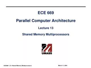
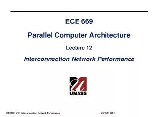
ECE 669 Parallel Computer Architecture Lecture 4 Parallel Applications. Outline. Motivating Problems (application case studies) Classifying problems Parallelizing applications Examining tradeoffs Understanding communication costs Remember: software and communication!. (a) Cross sections.

E N D
ECE 669Parallel Computer ArchitectureLecture 4Parallel Applications
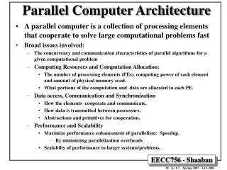
Outline • Motivating Problems (application case studies) • Classifying problems • Parallelizing applications • Examining tradeoffs • Understanding communication costs • Remember: software and communication!
(a) Cross sections Simulating Ocean Currents • Model as two-dimensional grids • Discretize in space and time • finer spatial and temporal resolution => greater accuracy • Many different computations per time step • set up and solve equations • Concurrency across and within grid computations • Static and regular (b) Spatial discretization of a cross section
Creating a Parallel Program • Pieces of the job: • Identify work that can be done in parallel • work includes computation, data access and I/O • Partition work and perhaps data among processes • Manage data access, communication and synchronization • Simplification: • How to represent big problem using simple computation and communication • Identifying the limiting factor • Later: balancing resources
4 Steps in Creating a Parallel Program • Decomposition of computation in tasks • Assignment of tasks to processes • Orchestration of data access, comm, synch. • Mapping processes to processors
Decomposition • Identify concurrency and decide level at which to exploit it • Break up computation into tasks to be divided among processors • Tasks may become available dynamically • No. of available tasks may vary with time • Goal: Enough tasks to keep processors busy, but not too many • Number of tasks available at a time is upper bound on achievable speedup
2n2 n2 + n2 p 2n2 2n2 + p2 Limited Concurrency: Amdahl’s Law • Most fundamental limitation on parallel speedup • If fraction s of seq execution is inherently serial, speedup <= 1/s • Example: 2-phase calculation • sweep over n-by-n grid and do some independent computation • sweep again and add each value to global sum • Time for first phase = n2/p • Second phase serialized at global variable, so time = n2 • Speedup <= or at most 2 • Trick: divide second phase into two • accumulate into private sum during sweep • add per-process private sum into global sum • Parallel time is n2/p + n2/p + p, and speedup at best
1 (a) n2 n2 p work done concurrently 1 (b) n2 n2/p p 1 (c) Time n2/p n2/p p Understanding Amdahl’s Law
fk k 1 k=1 1-s k s + fk p p k=1 Concurrency Profiles • Area under curve is total work done, or time with 1 processor • Horizontal extent is lower bound on time (infinite processors) • Speedup is the ratio: , base case: • Amdahl’s law applies to any overhead, not just limited concurrency
Applications • Classes of problems • Continuum • Particle • Graph, Combinatorial • Goal: Demystifying • Differential equations ---> Parallel Program
m1m2 r2 Particle Problems • Simulate the interactions of many particles evolving over time • Computing forces is expensive • Locality • Methods take advantage of force law: G • Many time-steps, plenty of concurrency across stars within one
Graph problems • Traveling salesman • Network flow • Dynamic programming • Searching, sorting, lists, • Generally unstructured
2 0 A B = Ñ + Continuous systems • Hyperbolic • Parabolic • Elliptic • Examples: • Heat diffusion • Electrostatic potential • Electromagnetic waves Laplace: B is zero Poisson: B is non-zero
Numerical solutions • Let’s do finite difference first • Solve • Discretize • Form system of equations • Solve ---> Result in system of equations • finite difference methods • finite element methods • . • . • . • Direct methods • Indirect methods • Iterative
1 x D = X grid points Discretize • Time • Where • Space • 1st • Where • 2nd • Can use other discretizations • Backward • Leap frog Forward difference n-2 Time n-1 n Boundary conditions Space A11 A12
1D Case • Or n + 1 n ] [ A 1 A - i i n n n A 2 A Ai-1 = - + + B i + 1 i 2 t D i x D 0 0
0 . . . . . . . . . . . . 0 Poisson’s For Or A x = b
A A . . . 22 21 2-D case • What is the form of this matrix? n A A A 11 12 13 . . .
Jacobi, ... Multigrid... . . . Iterative Direct Current status • We saw how to set up a system of equations • How to solve them • Poisson: Basic idea • In iterative methods • Iterate till no difference • The ultimate parallel method Or 0 for Laplace
In Matrix notation Ax= b • Set up a system of equations. • Now, solve • Direct: • Iterative: Gaussian elim. Recursive dbl. Direct methods Semi-direct - CG Iterative Jacobi MG Solve Ax=b directly LU Ax = b = -Ax+b Mx = Mx - Ax + b Mx = (M - A) x + b Mx k+1 = (M - A) xk + b Solve iteratively
Machine model • Data is distributed among memories (ignore initial I/O costs) • Communication over network-explicit • Processor can compute only on data in local memory. To effect communication, processor sends data to other node (writes into other memory). Interconnection network M M M P P P
Summary • Many types of parallel applications • Attempt to specify as classes (graph, particle, continuum) • We examine continuum problems as a series of finite differences • Partition in space and time • Distribute computation to processors • Understand processing and communication tradeoffs