Download
1 / 19
200 likes | 357 Vues
8. Project Management. PERT and CPM: techniques for planning and coordinating large-scale projects. PERT : program evaluation and review technique. CPM : Critical path method Graphically displays project activities Estimates how long the project will take Indicates most critical activities

E N D
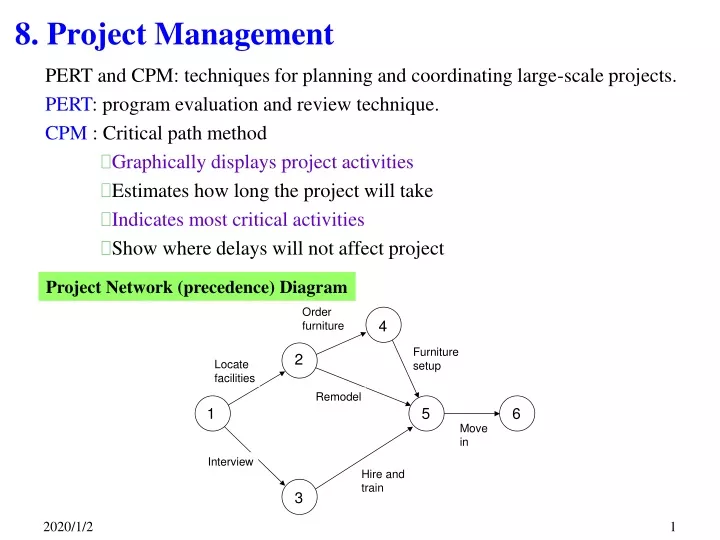
8. Project Management PERT and CPM: techniques for planning and coordinating large-scale projects. PERT: program evaluation and review technique. CPM : Critical path method • Graphically displays project activities • Estimates how long the project will take • Indicates most critical activities • Show where delays will not affect project Project Network (precedence) Diagram
8.1 Network Models of a Project AOA (Activity on Arrow model) The tasks (activities) are represented by arcs (arrows) in the network AON (Activity on Node model) The tasks (activities) are represented by the nodes in the network Example: A company is about to produce a product #3. One unit of product #3 is produced by assembling one unit of product #1(C) and one unit of product #2(D). Before production begins on either product #1 or #2, raw materials must be purchased (B) and workers must be trained (A). Before products #1 & #2 can be assembled into product #3 (F), the finished product #2 must be inspected (E).
8.1 Network Models of a Project - example B dummy 有彈性
4 6 weeks 2 3 weeks 8 weeks 11 weeks 1 5 6 1 week 4 weeks 9 weeks 3 Path Length Slack (weeks) 2 1-2-4-5-6 18 1-2-5-6 20 0 1-3-5-6 14 6 8.2 Deterministic time estimates Deterministic: Time estimates that are fairly certain Example of CPM: Computing Algorithm ES: the earliest time that activity can start. EF: the earliest time that activity can finish. LS: the latest time the activity can start and not delay the project. LF: the latest time the activity can finish and not delay the project. These for finding: • Expected project duration • Slack time • The activities on the critical path Steps of problem solving: labeling events computing ES and EF computing LS and LF computing Slack Times
8.3 Probabilistic time estimates Probabilistic : Estimates of times that allow for variation. Probabilistic Estimates - PERT One of the shortcomings of CPM is the assumption that the durations of activities are deterministic, i.e., known with certainty. PERT assume that the duration of each activity is random variable with known mean and standard variation, and derives a probability distribution for the project completion time. Assumptions of PERT The duration of an activity is a random variable with BETA distribution. The durations of the activities are statistically independent. The critical path (computed assuming expected values of the durations) always requires a longer total time than any other path. The Central Limit Theorem can be applied so that the sum of the durations of the activities on the critical path has approximately a NORMAL distribution.
8.3.1 Three time estimates • Optimistic time: represented by o • Pessimistic time: represented byp • Most likely time: represented by m It enables a manager to compute probabilistic estimates of the project completion time.
2-4-6 b 2-3-5 1-3-4 c a 5-7-9 3-5-7 3-4-5 e d f 2-3-6 3-4-6 g i 4-6-8 h 8.3.1 Three time estimates - example Example: • Compute the expected time for each activity and the expected duration for each path. • Identify the critical path. • Compute the variance of each activity and variance of each path.
Path Activity o m p te Path total (TE) N(TE,) a-b-c a b c 1 3 4 2 4 6 2 3 5 2.83 4.00 3.17 10.00 0.97 d-e-f d e f 3 4 5 3 5 7 5 7 9 4.00 5.00 7.00 16.00 1.00 N(16,1) g-h-i g h i 2 3 6 4 6 8 3 4 6 3.33 6.00 4.17 13.50 1.07 - - ì ü T 16 17 16 { } { } £ = £ = £ P T 17 P P X 1 í ý 1 1 î þ 8.3.1 Three time estimates - example The expected completion time of the project is 16 days. What is the probability that it is completed within 17 days?
8.4.1 Project Network (AOA) • A connected, directed network without circuits, with a unique source and unique sink. • The vertices are called "events“. • The arcs are called "activities", each with an associated nonnegative duration. Predecessors & Successors The project network indicates the order in which activities may be performed. Activity B cannot begin until activity A has been completed. • Activity A is a predecessor of activity B • Activity B is a successor of activity A
8.4.1 Project Network (AOA) - conventions 3 4 3 5 3 4 3
8.4.1 Project Network (AOA)– labeling events’ starting time for each activity ET(3) = 8 E C D B A
8.4.1 Project Network (AOA) – finding CPM For each activity, define: ES: the earliest time that activity can start. 最早可能的開始時間 EF: the earliest time that activity can finish. 最早可能的結束時間 LS: the latest time the activity can start and not delay the project. 最慢可能的start LF: the latest time the activity can finish and not delay the project.最慢可能的ending These for finding: • Expected project duration • Total slack (float) time and Free slack (float) • The activities on the critical path 不影響總時程的狀況下,每一項工作之 最大可能彈性時間 。 Steps of problem solving: • labeling events • computing ES and EF • computing LS and LF • computing Slack Times 每一項後續工作,都準時開始的狀況下, 最大可能彈性時間。(即不影響ET(j)的意思)
8.4.1 Project Network (AOA) – TF & FF EF(1,3) ES(1,3) LS(1,3) A LF(1,3) FF(3,4) = 14 – 3 – 10 = 1 TF(1,3) 14 LS(2,3) LF(2,3) 4 C 3 10 B 0 A 2 EF(2,3) ES(2,3) 3 LF(3,4) 1 9 E ES(3,4) LS(3,4) B 5 D 5 C EF(3,4) 11 2 D 5 E 10 14 5 2 13 FF(2,4) = 14 –9 – 5 = 0 0 TF(3,4) TF(2,3) TF(1,2), TF(2,4) = 0
0 8.4.1 Project Network (AOA) – TF & FF – example 10 14 TFFF 0 (0,1) (1,2) (0,3) (2,4) (3,5) (4,6) (4,7) (5,7) (1,8) (7,8) 8
8.5 Project Network (AON) -Linear Programming Model Define Yx = starting time (i.e.,ET(x)) for activity x Objective: Minimize Yend - Ybegin Constraints: For every predecessor requirement, we will have an inequality constraint:For example, “A must precede C” translates to where dA is the duration of activity A.
C 4 1 A F D 0 5 E B Begin End 3 2 8.5 Project Network (AON) -Linear Programming Model cont’s yA yBegin yB yBegin yC yA+dA yC yB+dB . . .
11 15 4 3 4 1 C 9/540 *7/600 A 4/210 *3/280 H 7/600 *6/750 D 6/500 *4/600 ET(0)=0 ET(0)=0 22 17 E 5/150 *4/240 5 0 End Begin G 3/150 *3/150 B 8/400 *6/560 3 2 F 4/500 *1/1100 ? 14 7 10 540+(600-540)/(9-7) 8.6 Project Cost 成 本 11 4500- - - - - 4000- - - - - 3500- - - - - 3000- 4280 4080 3870= 210+560+600+500+150+1100+150+600 可能的 直接成本區 CPM (A→D→E→H)之最短時程為17天:成本1870 此時A→C→H時程為18天故C趕工1天:成本570 而B→E→H的B要趕工1天:成本1130總成本:3570 - - - - - - 3570 3260 3050 = 210+400+540+500+150+500+150+600 工作天 17 18 19 20 21 22
5910 5850- - - - - 5800- - - - - 5750- - - - - 5700- 總成本 成 本 5780 - - - - - - 5730 17 18 19 20 21 22 直接成本 3570 3500- - - - - 3000- - - - - 2500- - - - - 2000- 3420 3100 3260 3050 3170 2730 2860 2600 2470 假設每一工作每縮短一天之成本為其 總增加成本 最多縮短天數 - - - - - - 2340 間接成本 130/日 2210 工作天 17 18 19 20 21 22 8.6 Project Cost – cont’s Min 130×(yEnd-yBegin) -(70dA+80dB+30dC+50dD+90dE+200dF+150dH) Min 210+400+540+500+150+500+150+600+70(4-dA)+80(8-dB) +30(9-dC)+50(6-dD)+90(5-dE)+200(4-dF)+150(7-dH)+130×(yEnd-yBegin) = 6840- (70dA+80dB+30dC+50dD+90dE+200dF+150dH) +130×(yEnd-yBegin) Minimize ??? yA yBegin; yEnd yH+dH yB yBegin ; yEnd yG+dG yC yA+dA; 3 dA 4 yD yA+dA; 6 dB 8 yE yB+dB; 7 dC 9 yE yD+dD; 4 dD 6 yF yB+dB;4 dE 5 yF yD+dD; 1 dF 4 yH yC+dC; dG= 3 yH yE+dE; 6 dH 7 yG yF+dF