Download
1 / 102
1.3k likes | 1.61k Vues
Network Analyzer Basics. Author: David Ballo. Router. Bridge. Repeater. Hub. Your IEEE 802.3 X.25 ISDN switched-packet data stream is running at 147 MBPS with a BER of 1.523 X 10. -9. Network analysis is not. What types of devices are tested?. Duplexers Diplexers Filters Couplers

E N D
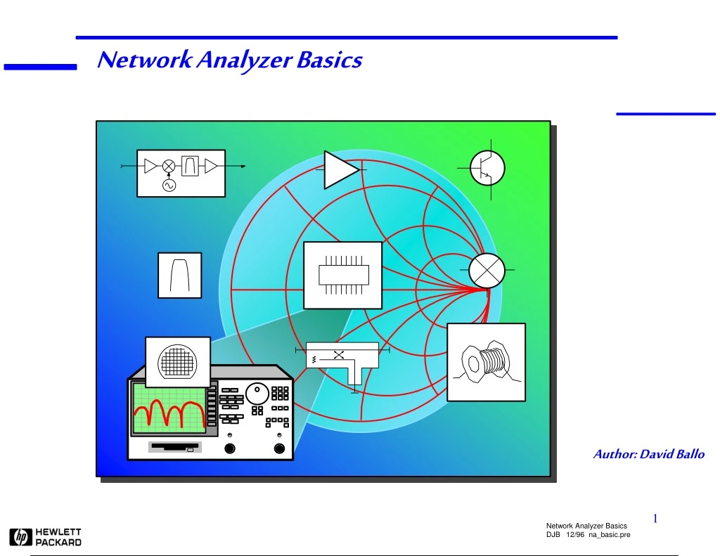
Network Analyzer Basics Author: David Ballo
Router Bridge Repeater Hub Your IEEE 802.3 X.25 ISDN switched-packet data stream is running at 147 MBPS with a BER of 1.523 X 10 . . . -9 Network analysis is not...
What types of devices are tested? Duplexers Diplexers Filters Couplers Bridges Splitters, dividers Combiners Isolators Circulators Attenuators Adapters Opens, shorts, loads Delay lines Cables Transmission lines Waveguide Resonators Dielectrics R, L, C's RFICs MMICs T/R modules Transceivers Receivers Tuners Converters VCAs Amplifiers VCOs VTFs Oscillators Modulators VCAtten's Transistors High Integration Antennas Switches Multiplexers Mixers Samplers Multipliers Diodes Low Device type Active Passive
Measurement plane DC CW Swept Swept Noise 2-tone Multi- Complex Pulsed- Protocol freq power tone modulation RF Device Test Measurement Model 84000 RFIC test Full call sequence BER EVM ACP Regrowth Constell. Eye Complex Ded. Testers Pulsed S-parm. Pulse profiling VSA Harm. Dist. LO stability Image Rej. Intermodulation Distortion NF SA Gain/Flat. Phase/GD Isolation Rtn Ls/VSWR Impedance S-parameters Compr'n AM-PM VNA TG/SA Response tool SNA NF Mtr. NF Imped. An. LCR/Z Param. An. I-V Simple Absol. Power Power Mtr. Det/Scope Gain/Flatness Stimulus type Simple Complex
Agenda • Why do we test components? • What measurements do we make? • Smith chart review • Transmission line basics • Reflection and transmission parameters • S-parameter definition • Network analyzer hardware • Signal separation devices • Broadband versus narrowband detection • Dynamic range • T/R versus S-parameter test sets • Three versus four samplers • Error models and calibration • Types of measurement error • One- and two-port models • Error-correction choices • TRL versus TRL* • Basic uncertainty calculations • Typical measurements • Advanced topics
Why do we need to test components? Components often used as building blocks • Need to verify specifications • Examples: • filters to remove harmonics • amplifiers to boost LO power • mixers to convert reference signals When used to pass communications signals, need to ensure distortionless transmission • Linear networks • constant amplitude • linear phase / constant group delay • Nonlinear networks • harmonics, intermodulation • compression • noise figure When absorbing power (e.g. an antenna), need to ensure good match
A * Sin 360 * f ( t - t ) ° ° Sin 360 * f * t A ° phase shift = to * 360 * f ° f Time Frequency 1 DUT f 1 f 1 Linear Versus Nonlinear Behavior Linear behavior: • input and output frequencies are the same (no additional frequencies created) • output frequency only undergoes magnitude and phase change A Time t o Input Output Nonlinear behavior: • output frequency may undergo frequency shift (e.g. with mixers) • additional frequencies created (harmonics, intermodulation) Frequency Time Frequency
Criteria for Distortionless Transmission Linear Networks Constant amplitude over bandwidth of interest Linear phase over bandwidth of interest Magnitude Phase Frequency Frequency
Linear Network Network Analyzer Basics DJB 12/96 na_basic.pre Magnitude Variation with Frequency F(t) = sin wt + 1 /3 sin 3wt + 1 /5 sin 5wt H Time Time Magnitude Frequency Frequency Frequency
Phase Variation with Frequency F(t) = sin wt + 1 /3 sin 3wt + 1 /5 sin 5wt Linear Network Time Time Magnitude Frequency 0 ° Frequency Frequency -180 ° -360 °
Time Time Frequency Frequency Criteria for Distortionless Transmission Nonlinear Networks Saturation, crossover, intermodulation, and other nonlinear effects can cause signal distortion
KPWR KPWR FM 97 FM 97 Example Where Match is Important Wire and bad antenna (poor match at 97 MHz) results in 150 W radiated power Proper transmission line and antenna results in 1500 W radiated power - signal is received about three times further! Good match between antenna and RF amplifier is extremely important to radio stations to get maximum radiated power
S 21 Complete characterization of linear networks 1. S S 11 22 S 12 Error Collector Base Measured Emitter Actual The Need for Both Magnitude and Phase Time Domain Characterization 4. Complex impedance needed to design matching circuits Mag 2. Time High Frequency Transistor Model Vector Accuracy Enhancement 5. Complex values needed for device modeling 3.
Why do we test components? • What measurements do we make? • Network analyzer hardware • Error models and calibration • Typical measurements • Advanced topics Agenda
Incident Transmitted Reflected High-Frequency Device Characterization Lightwave Analogy
o +jX 90 +R 0 ¥ o + o 180 0 - ¥ 0 -jX o -90 Smith Chart Review . Polar plane 1.0 .8 .6 .4 .2 Rectilinear impedance plane Constant X Z = Zo Constant R L G = 0 Smith Chart maps rectilinear impedance plane onto polar plane (short) (open) Z = 0 Z = L L G G O 0 = 1 O 1 ±180 = Smith Chart
RS RL Power Transfer For complex impedances, maximum power transfer occurs when ZL = ZS* (conjugate match) Zs = R +jX RL / RS ZL= Zs* = R -jX Maximum power is transferred when RL = RS
Transmission Line Review I Low frequencies • Wavelength >> wire length • Current (I) travels down wires easily for efficient power transmission • Voltage and current not dependent on position High frequencies • Wavelength » or << wire (transmission line) length • Need transmission-line structures for efficient power transmission • Matching to characteristic impedance (Z0) is very important for low reflection • Voltage dependent on position along line
Zo = characteristic impedance of transmission line Zs = Zo Zo V inc Vrefl = 0! (all the incident power is absorbed in the load) Transmission Line Terminated with Zo For reflection, a transmission line terminated in Zo behaves like an infinitely long transmission line
V inc o In phase (0 ) for open Out of phase (180 ) for short o Transmission Line Terminated with Short, Open Zs = Zo Vrefl For reflection, a transmission line terminated in a short or open reflects all power back to source
V inc Transmission Line Terminated with 25 W Zs = Zo ZL = 25 W Vrefl Standing wave pattern does not go to zero as with short or open
Incident Transmitted Reflected B Transmitted A Reflected = = R Incident R Incident High-Frequency Device Characterization R B A TRANSMISSION REFLECTION Group Return SWR Gain / Loss Delay Loss Insertion S-Parameters Impedance, Admittance S-Parameters S11,S22 Phase Reflection Transmission S21,S12 Coefficient R+jX, G+jB Coefficient G, r T,t
- r V Z Z Reflection F reflected O L Coefficient V Z Z + incident O L Emax 1 + r Emax Emin VSWR = = 1 - r Emin Reflection Parameters G = = = r Return loss = -20 log(r), G = Voltage Standing Wave Ratio Full reflection (ZL = open, short) No reflection (ZL = Zo) r 1 0 ¥dB 0 dB RL ¥ 1 VSWR
V Transmitted DUT V Transmission Coefficient = T Transmitted = tÐf = V Incident V Trans V Inc V Gain (dB) = 20 Log = 20 log t Trans V Inc Transmission Parameters V Incident = - 20 log t Insertion Loss (dB) = - 20 Log
o o Phase 45 /Div Phase 1 /Div Deviation from Linear Phase Use electrical delay to remove linear portion of phase response Linear electrical length added Deviation from linear phase RF filter response (Electrical delay function) + yields Frequency Frequency Frequency Low resolution High resolution
-d f d w d f d f p w ( f ) 2 = What is group delay? Group Delay w t g Frequency Group Dw Delay t o f Phase Average Delay Df Group Delay (t ) = Frequency g Deviation from constant group delay indicates distortion -1 = * o 360 f in radians Average delay indicates transit time w in radians/sec f in degrees in Hz f
-d f -d f d w d w Why measure group delay? Phase Phase f f Group Delay Group Delay f f Same p-p phase ripple can result in different group delay
V1 h11 = I1 V2=0 Low-Frequency Network Characterization H-parameters V1 = h11I1 + h12V2 V2 = h21I1 + h22V2 Y-parameters I1 = y11V1 + y12V2 I2 = y21V1 + y22V2 Z-parameters V1 = z11I1 + z12I2 V2 = z21I1 + z22I2 (requires short circuit) V1 h12 = V2 (requires open circuit) I1=0 All of these parameters require measuring voltage and current (as a function of frequency)
S 21 Incident Transmitted a 1 b 2 S 11 DUT Reflected S 22 Port 2 Port 1 Reflected a b 2 1 Incident S Transmitted 12 b a a S = S + 1 11 12 2 1 b a = a S S + 2 21 22 2 1 Limitations of H, Y, Z Parameters (Why use S-parameters?) H,Y, Z parameters • Hard to measure total voltage and current at device ports at high frequencies • Active devices may oscillate or self-destruct with shorts / opens S-parameters • Relate to familiar measurements (gain, loss, reflection coefficient ...) • Relatively easy to measure • Can cascade S-parameters of multiple devices to predict system performance • Analytically convenient • CAD programs • Flow-graph analysis • Can compute H, Y,or Z parameters from S-parameters if desired
b S 2 Incident Transmitted 21 a 1 Z S 0 Forward 11 Load DUT Reflected b a 0 = 1 2 b Reflected 1 S = = 11 a a Incident 0 = b 1 2 Reflected 2 S = = b 22 a a Transmitted Incident 0 = 2 S 1 2 = = 21 a a 0 = b Incident 2 Transmitted 1 S 1 = = 12 a a 0 = Incident 1 2 a b 0 = 1 2 S Z 22 Reverse DUT 0 Reflected Load a 2 S Transmitted Incident 12 b 1 Measuring S-Parameters
RL 0 dBm ATTEN 10 dB 10 dB / DIV 8563A SPECTRUM ANALYZER 9 kHz - 26.5 GHz LPF DUT CENTER 20.00000 MHz SPAN 10.00 kHz RB 30 Hz VB 30 Hz ST 20 sec LPF Measuring Nonlinear Behavior Most common measurements: • Using a spectrum analyzer + source(s) • harmonics, particularly second and third • intermodulation products resulting from two or more carriers • Using a network analyzer and power sweeps • gain compression • AM to PM conversion • Noise figure
8563A SPECTRUM ANALYZER 9 kHz - 26.5 GHz Power Frequency Spectrum analyzers: • measure signal amplitude characteristics (carrier level, sidebands, harmonics...) • are receivers only (single channel) • can be used for scalar component test (no phase) with tracking gen. or ext. source(s) Network analyzers: • measure components, devices, circuits, sub-assemblies • contain source and receiver • display ratioed amplitude and phase (frequency or power sweeps) What is the difference between network and spectrum analyzers? . Hard: getting (accurate) trace Easy: interpreting results Easy: getting trace Hard: interpreting results Amplitude Ratio Measures unknown signals Measures known signal Frequency
Why do we test components? • What measurements do we make? • Network analyzer hardware • Error models and calibration • Typical measurements • Advanced topics Agenda
Incident Transmitted DUT Reflected SOURCE SIGNAL SEPARATION INCIDENT (R) REFLECTED (A) TRANSMITTED (B) RECEIVER / DETECTOR PROCESSOR / DISPLAY Generalized Network Analyzer Block Diagram H
Source • Supplies stimulus for system • Swept frequency or power • Traditionally NAs used separate source • Open-loop VCOs • Synthesized sweepers • Most HP analyzers sold today have integrated, synthesized sources Integrated, synthesized sources
6 dB 50 W 6 dB 50 W Signal Separation Measuring incident signals for ratioing • Splitter • usually resistive • non-directional • broadband • Coupler • directional • low loss • good isolation, directivity • hard to get low freq performance Main signal Coupled signal
Detector Test Port Signal Separation Separating incident and reflected signals • Coupler • directional • low loss • good isolation, directivity • hard to get low freq performance • Bridge • used to measure reflected signals only • broadband • higher loss
Forward Coupling Factor Coupling, forward -20 dBm .01 mW Source Z 0 -.046 dBm 0 dBm 1 mW .99 mW Example of 20 dB Coupler coupling forward P Coupling Factor (dB) = -10 log P incident
Source P coupled reverse P incident Directional Coupler Isolation (Reverse Coupling Factor) Coupling, reverse -50 dBm this is an error signal during measurements .00001 mW Z 0 0 dBm 1 mW -.046 dBm .99 mW Example of 20 dB Coupler "turned around" Isolation Factor (dB) = -10 log
P coupled forward P coupled reverse Coupling Factor Directivity = Isolation Directional Coupler Directivity Directivity (dB) = 10 log Directivity (dB) = Isolation (dB) - Coupling Factor (dB) Example of 20 dB Coupler with 50 dB isolation: Directivity = 50 dB - 20 dB = 30 dB
Coupler Directivity 35 dB short Source load Measuring Coupler Directivity the Easy Way 1.0 (0 dB) (reference) Good approximation for coupling factors ³10 dB .018 (35 dB) (normalized) Directivity = 35 dB - 0 dB = 35 dB Source Assume perfect load
Device Directivity Interaction of Directivity with the DUT (Without Error Correction) 0 Data Max DUT RL = 40 dB Add in Phase Directivity 30 Device Return Loss 60 Frequency Device Data Min Data = Vector Sum Directivity Cancel Data » 0
Directional Bridge • 50 ohm load at test port balances the bridge - detector reads zero • Extent of bridge imbalance indicates impedance • Measuring magnitude and phase of imbalance gives complex impedance • "Directivity" is difference between maximum and minimum balance 50 W 50 W Detector Test Port 50 W
Incident Transmitted DUT Reflected SOURCE SIGNAL SEPARATION INCIDENT (R) REFLECTED (A) TRANSMITTED (B) RECEIVER / DETECTOR Diode PROCESSOR / DISPLAY Scalar broadband (no phase information) DC RF AC Tuned Receiver Scalar narrowband (magnitude only) RF ± IF = F F LO RF ADC / DSP Vector (magnitude and phase) IF Filter LO Detector Types
26.5 GHz 10 MHz Broadband Diode Detection • Easy to make broadband • Inexpensive compared to tuned receiver • Good for measuring frequency-translating devices • Improve dynamic range by increasing power • Medium sensitivity / dynamic range
ADC / DSP Narrowband Detection - Tuned Receiver • Best sensitivity / dynamic range • Provides harmonic / spurious signal rejection • Improve dynamic range by increasing power, decreasing IF bandwidth, or averaging • Trade off noise floor and measurement speed 10 MHz 26.5 GHz
Sampler-based front end S ADC / DSP ADC / DSP f Harmonic generator frequency "comb" Front Ends: Mixers Versus Samplers Mixer-based front end It is cheaper and easier to make broadband front ends using samplers instead of mixers
0 dB -50 dB -100 dB Comparison of Receiver Techniques Broadband (diode) detection Narrowband (tuned- receiver) detection 0 dB -50 dB -100 dB -60 dBm Sensitivity < -100 dBm Sensitivity • higher noise floor • false responses • high dynamic range • harmonic immunity Dynamic range = maximum receiver power - receiver noise floor
RF R A B RF R A B DUT DUT Traditional Scalar Analyzer Traditional scalar system consists of processor/display and source Example: HP 8757D • requires external detectors, couplers, bridges, splitters • good for low-cost microwave scalar applications Detector Detector Detector Bridge Termination Reflection Transmission