Download
1 / 51
510 likes | 606 Vues
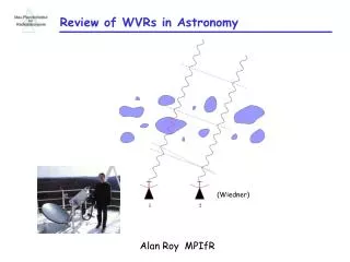
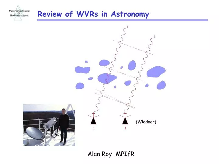
Review of WVRs in Astronomy. (Wiedner). Alan Roy MPIfR. The Troposphere as Seen from Orbit. Method: Synthetic Aperture Radar (Earth Resources Satellite) Frequency: 9 GHz Region: Groningen Interferograms by differencing images from different days. 100 mm. 0 mm. 5 km. -100 mm.

E N D
Review of WVRs in Astronomy (Wiedner) Alan Roy MPIfR
The Troposphere as Seen from Orbit Method: Synthetic Aperture Radar (Earth Resources Satellite) Frequency: 9 GHz Region: Groningen Interferograms by differencing images from different days 100 mm 0 mm 5 km -100 mm A frontal zone Convective cells 5 km Internal waves in a homo- genously cloudy troposphere Hanssen (1997)
Coherence Loss due to Troposphere VLBI phase time series Coherence Function 360° 7 min Pico Veleta – Onsala baseline Source: BL Lac Frequency: 86 GHz
WVR Performance Requirements Phase Correction Aim: coherence = 0.9 requires / 20 (0.18 mm rms at = 3.4 mm) after correction Need: thermal noise 14 mK in 3 s Need: gain stability 3.9 x 10⁻⁴ in 300 s Zenith Delay for Phase Referencing Aim: transfer phase over 5o with 0.1 rad error at 43 GHz Need: absolute ZWD with error < 1 mm (?)
WVR Performance Requirements Opacity Measurement Aim: correct visibility amplitude to 1 % (1 ) Need: thermal noise 2.7 K Need: absolute calibration 14 % (1 )
Phase Correction Methods • Use a nearby strong calibrator • a) Interleave source and calibrator observations • BUT: must cycle fast -> short integrations -> few calibrators strong enough • b) Dual beam: observe simultaneously calibrator and source (VERA) • BUT: need duplicate moveable receiver • c) Dual frequency: observe target source at lower frequency scale up • phase to calibrate the higher frequency • BUT: scaling up multiplies the phase noise; • need very good low-frequency observation • d) Paired antennas: one observes target, one observes calibrator (Asaki 1997) • Measure the water vapour and infer the phase • a) Total power method • b) Radiometric phase correction (eg at 22 GHz, 183 GHz or 20 um)
WVR Phase Correction Performance Comparison Telescope Technique Freq Path Residual / mm dG/G dT in 1 s VLA WLM 22 GHz cooled 0.81 0.6x10⁻⁴(100 s) 20 mK Plateau de Bure WLM 22 GHz uncooled 0.031 7.5x10⁻⁴ (30 min) Plateau de Bure TP 230 GHz cooled 0.041 2x10⁻⁴ Pico Veleta TP 230 GHz cooled 0.24 OVRO WLM 22 GHz uncooled 0.16 10 mK BIMA TP 90 GHz cooled 0.17 BIMA WLM 22 GHz uncooled 0.1 5x10⁻³ CSO-JCMT WLM 183 GHz uncooled 0.06 SMA TP 230 GHz cooled 0.09 2x10⁻⁴ SMA WLM 183 GHz uncooled ATCA WLM 22 GHz cooled 0.3 12 mK Effelsberg WLM 22 GHz uncooled 0.24 5x10⁻⁴(100 s) 12 mK VLBA TP 86 GHz cooled 0.6 Chatnantor WLM 183 GHz uncooled 0.08 2x10⁻³ (100s) DSN WLM 22 GHz uncooled 0.21 25 mK (8 s) IRMA WLM 15 THz cooled = represented at this meeting = lowest rms phase demonstrated
Total Power Phase Correction Plateau de Bure Total power at 230 GHz Correction applied to simultaneous 90.6 GHz Phase correction 3 mm Observed phase: rms = 0.623 mm Corrected phase: rms = 0.167 mm 30 min Bremer 1995, 2000
Total Power Phase Correction: VLBI demo Pico Veleta - Onsala Total power at 230 GHz Correction applied to simultaneous 86 GHz VLBI Observed phase: rms = 0.71 mm 4.7 mm Phase correction Corrected phase: rms = 0.45 mm 6 min Bremer et al. 2000
Owens Valley Radio Observatory (Caltech) (Array before moving to Cedar Flat) Frequencies: 86 - 115 GHz 210 – 270 GHz Antenna diam: 10.4 m Altitude: 1220 m
Owens Valley Radio Observatory Woody, Carpenter, Scoville 2000, ASP Conf Ser 217, 317 Downconvert to 4 GHz to 12 GHz (cheaper components, better characterized) Uncooled LNA (Tsys = 200 K) Cold load (optional) 363 K load Ambient load Analog difference of line and continuum channels Analog sum of wing channels for continuum Triplexer separates 2 GHz Bands on line and off-line 18.2 to 20.2, 21.2 to 23.2, 24.2 to 26.2 GHz to 16-bit A/D Alternate L and C every 1.7 ms
Owens Valley Radio Observatory • Two levels of Dicke switching reduce effects of gain and offset drifts: • 1) PIN-diode attenuators adjust the Line-Continuum output to be zero • for blackbody loads; output measures deviation from a flat spectrum. • Transfer switch reverses assignment of Line and Continuum to the • detectors every 1.7 ms; demodulation is performed in software • -> removes DC offsets and most of the gain drifts in detectors and following • electronics • Results: • Allan Variance -> noise in L - C < 10 mK for 20 s to 20 min • while noise in L & C > 30 mK • -> analog L – C differencing and transfer switch modulation valuable • C1 & C2 channels derived from -10 dB coupler have 10x more noise • -> standard radiometer noise is not the dominant noise • White noise to 1 s in L or C channels separately • White noise to 10 s in L-C channel Woody et al. (2000)
Owens Valley Radio Observatory Calibration Once per hour hot & ambient load Solve for gain, Tsys, and drift in offset of L-C channel Accuracy of gain determination: 1 % Noise in offset determination: 20 mK Woody et al. (2000)
Owens Valley Radio Observatory interferometer path at 100 GHz WVR predicted path 3 mm RMS before correction = 0.53 mm RMS after correction = 0.16 mm 26 min Woody et al. (2000)
Owens Valley Radio Observatory Path Length Retrieval Observe a strong calibrator -> conversion factor Typically use a fixed 12 mm/K cf calculated conversion factor of 8 mm/K Difference is “within the uncertainties of the triplexer bandpass shapes and atmospheric model assumptions” Woody et al. (2000)
Owens Valley Radio Observatory Woody et al. (2000)
Owens Valley Radio Observatory Transferring phase between calibrator and source: hard! (due to gradient in sky brightness) must normalize gains among the WVRs using the step due to elevation change L-C from each WVR / K Average L-C from all WVRs / K Woody et al. (2000)
Owens Valley Radio Observatory 0309+411 at 100 GHz for 5 h Cycle: 6 min source, 6 min calibrator (0.7 degrees away) WVR phase is transferred from calibrator to source Before WVR correction (good weather) (weather degraded) 28 Jy 36 Jy 13 Jy After WVR correction 40 Jy 42 Jy 34 Jy Woody et al. (2000)
Owens Valley Radio Observatory Conclusion Can correct tropospheric phase fluctuations down to < 0.2 mm. Allows 3 mm observations in previously unusable weather. Not sufficient for improving images during typical conditions Or for routine use during 1 mm observations. Developing a cooled version to decrease noise to reach 0.05 mm. Staguhn et al. 2001, ASP Conf: First light on prototype Cooled 22 GHz WVR Double sideband heterodyne 0.5 GHz to 4 GHz IF 16 channel analogue lag correlator (APHID) (see Alberto Bolatto’s talk) Woody et al. (2000)
JCMT – CSO Interferometer James Clark Maxwell Telescope (JCMT) Caltech Submillimeter Observatory (CSO) Frequencies: 210 – 270 GHz 318 – 360 GHz Higher than OVRO 460 – 500 GHz Antenna diam: 10.4 m & 15 m Altitude: 4092 m Higher than OVRO Location: Hawaii
JCMT – CSO: 183 GHz WVRs Wiedner 1998 PhD thesis Wiedner, Hills, Carlstrom, Lay 2001, ApJ, 553, 1036 Line pivot points: least sensitive to altitude of water vapour
JCMT – CSO: 183 GHz WVRs Wiedner 1998 PhD thesis Wiedner, Hills, Carlstrom, Lay 2001, ApJ, 553, 1036 The three double-sideband frequency channels of the WLM
JCMT – CSO: 183 GHz WVRs Wiedner 1998 PhD thesis Wiedner, Hills, Carlstrom, Lay 2001, ApJ, 553, 1036 Advantages of 183 GHz over 22 GHz: - line is 10 x stronger than 22 GHz. -> can build uncooled systems - optics are small -> easier to install in existing telescopes Disadvantages of 183 GHz: - line saturates easily -> suitable only for dry sites - retrieval coefficient depends on amount of water vapour and conditions
JCMT – CSO: 183 GHz WVRs Wiedner 1998 PhD thesis Wiedner, Hills, Carlstrom, Lay 2001, ApJ, 553, 1036
JCMT – CSO: 183 GHz WVRs Wiedner 1998 PhD thesis Wiedner, Hills, Carlstrom, Lay 2001, ApJ, 553, 1036 Calibration - Loads at 30 C and 100 C - Load stability: 10 mK - Flip mirror cycles every 1 s between sky and loads Load temperature vs time 10 mK Sectioned drawing of load 5 min
JCMT – CSO: 183 GHz WVRs Wiedner 1998 PhD thesis Wiedner, Hills, Carlstrom, Lay 2001, ApJ, 553, 1036 Mirror 2 Mirror 1 Warm load Hot load Corrugated horn (facing away)
JCMT – CSO: 183 GHz WVRs Wiedner 1998 PhD thesis Wiedner, Hills, Carlstrom, Lay 2001, ApJ, 553, 1036 Uncooled mixer (Tsys = 2500 K) 183.31 GHz +/- 8 GHz Coupler Power splitter Mixer Filter Detector V/F Used coupler + power splitter since no suitable triplexer exists 1.2 GHz 4.2 GHz 7.8 GHz Oscillators Double-sideband mixing makes measurement insensitive to filter shape Gunn oscillator 91.655 GHz
JCMT – CSO: 183 GHz WVRs Wiedner 1998 PhD thesis Wiedner, Hills, Carlstrom, Lay 2001, ApJ, 553, 1036 A small shift in the centre frequency of a filter makes a big change in the measured brightness temperature since the line is steep. Thus, need filter shape within 5 MHz of spec. No triplexer matched this.
JCMT – CSO: 183 GHz WVRs Wiedner 1998 PhD thesis Wiedner, Hills, Carlstrom, Lay 2001, ApJ, 553, 1036 DSB mixing to baseband folds water line at oscillator frequency Result is flat water line spectrum Water line spectrum is then same as the calibration load spectrum Calibration factor is then independent of the filter shape
JCMT – CSO: 183 GHz WVRs Wiedner 1998 PhD thesis Wiedner, Hills, Carlstrom, Lay 2001, ApJ, 553, 1036 WVR at CSO (outside, so less stable environment) 10x10-4 2x10⁻⁴ WVR at JCMT 9 min Gain fluctuations of WVR measured against loads each second
JCMT – CSO: 183 GHz WVRs Wiedner 1998 PhD thesis Wiedner, Hills, Carlstrom, Lay 2001, ApJ, 553, 1036 Maser source MWC 349 at 356 GHz WVR correction Before correction RMS = 127d = 0.30 mm 1.4 mm After correction RMS = 48d = 0.11 mm 12 min Atmospheric model: transition strengths from Waters (1976), Ben-Reuven line profile, exponential atmosphere, radiative transfer calculation
Sub-Millimeter Array CSO JCMT SMA 183 GHz WVRs being installed. (Talks by Ross Williamson & Richard Hills)
Very Large Array Dave Finley Image courtesy NRAO/AUI 22 GHz WVRs being prototyped. (Talk by Walter Brisken)
Plateau de Bure 22 GHz WVRs in routine operation. (Talks by Michael Bremer & Aris Karastergiou)
Effelsberg 22 GHz sweeping WVR operating. (Talk by Alan Roy)
Berkeley-Illinois-Maryland Array 22 GHz sweeping WVRs prototyped. Array relocated to Cedar Flat with OVRO antennas Now called CARMA. (Talk by Alberto Bolatto)
VLBI Phase Correction Demo Demonstration by Tahmoush & Rogers (2000) 3C 273 Hat Creek – Kitt Peak 86 GHz VLBI path 4 mm VLBI phase WVR phase 400 s ● RMS phase noise reduced from 0.88 mm to 0.34 mm after correction. ● Coherent SNR rose by 68 %.
CARMA Jim Stimson Photography (Talk by Alberto Bolatto)
Chajnantor Site Testing Two 183 GHz WVRs 300 m apart Duplicates of JCMT-CSO WVRs (Hills/Wiedner) Co-located with two 11.2 GHz seeing interferometers observing a geostationary satellite Delgado et al. 2001, ALMA Memo 361
Chajnantor Site Testing Correlation coefficient between WVR and interferometers varied. Cause: when turbulence is lower than 300 m it lies in near-field of interferometer antennas causing large beam differences between the instruments (?) Delgado et al. 2001, ALMA Memo 361
Chajnantor Site Testing Delgado et al. 2001, ALMA Memo 361
Chajnantor Site Testing Delgado et al. 2001, ALMA Memo 361
Australia Telescope Compact Array Frequencies: 1.2 - 106 GHz Antenna diam: 22 m Altitude: 300 m
NASA Deep Space Network 22 GHz to 32 GHz WVR (Tanner et al.) For Cassini gravity wave experiment Naudet et al. (2000)
NASA Deep Space Network Need: 10 mK radiometric stability from 100 s to 10000 s Focus: improve precision and stability of noise diode and Dicke switch Methods: 1) Regulate temperature in radiometer box to 1 mK. 2) bought commercial noise diodes. 3) follow instructions to bias with regulated 28 V. -> poor stability: 20 x 10-4 in 10 s - 100 s 4) try current-regulating bias circuit -> immediate improvement to 1 x 10⁻⁴ in 100 s, 5 x 10⁻⁴ in 1 day 5) replace magic T power combiner with directional couplers due to extreme sensitivity to mismatch (-40 dB reflection caused 4 % change of noise diode power) -> 1 x 10⁻⁴ in 1 day 6) regulate the relative humidity -> 0.3 x 10⁻⁴ in 1 day 7) Dicke switch using absorber inserted in slotted waveguide by loudspeaker voicecoil Tanner et al. (1998)
NASA Deep Space Network 2 mm 4 h RMS before correction = 0.43 mm RMS after correction = 0.1 mm Naudet et al. (2000)