Download
1 / 41
500 likes | 790 Vues
Network Topologies. William M. Jones Assistant Professor Computer Science Department Coastal Carolina University. Network Classifications. Networks have two broad classifications Static Dynamic Static Networks

E N D
Network Topologies William M. Jones Assistant Professor Computer Science Department Coastal Carolina University
Network Classifications • Networks have two broad classifications • Static • Dynamic • Static Networks • Static networks consist of point-to-point communication links among nodes and are also referred to as direct networks • Dynamic Networks • Dynamic networks are built using switches and communication links. Dynamic networks are also referred to as indirect networks. For example ….
The only non-PC, networking devices are adjacent to the PCs themselves Networking devices are potentially non-adjacent to the PCs.
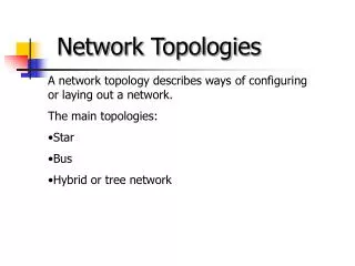
Network Topologies • A variety of network topologies have been proposed and implemented • These topologies tradeoff performance for cost; a full analysis goes beyond the scope of this course • Commercial machines often implement hybrids of multiple topologies for reasons of packaging, cost, and available components Let’s take a look at some common static network topologies …
Linear Arrays (1D) What happens if link is cut? Susceptible to congestion Bus Ring What are some of the drawbacks here?
Meshes (2D, 3D) 2 links cut 4 links cut More connectivity better fault tolerance more cost Two and three dimensional meshes: (a) 2-D mesh with no wraparound; (b) 2-D mesh with wraparound link (2-D torus); and (c) a 3-D mesh with no wraparound. In terms of graph theory, networks can be described by a set of vertices (nodes) and a set of edges (links) What’s up with these topologies? 4+ NW wires / PC, I’ve never seen a computer like that before!
Hypercubes (4D) To just add one more computer to network requires doubling the number of computers Adding only one additional node severely disrupts symmetry
Note that the vertices can be numbered so that the Hamming distance between any two adjacent vertices is 1. This plays an important role in determining a path from sender to receiver (i.e. routing). For example …
Source Dest. Suppose node 0101 wants to send a message to node 1111. Starting with the LSB of the numbers, compare the destination address bit to the sending address bit and if they are different, take the adjacent link that makes them the same. This is referred to as dimension order routing.
Source Dest. Step 1 -- 0101 to 1111: These are the same do nothing
Source Dest. Step 1 -- 0101 to 1111: These are the same do nothing Step 2 -- 0101 t0 1111: These are different follow the edge that takes you to a vertex that is 0111 – (a given node only has to know the address of his neighbors to make this work, which is a nice simplification)
Source Dest. Step 1 -- 0101 to 1111: These are the same do nothing, go to next bit Step 2 -- 0101 to 1111: These are different follow the edge that takes you to a vertex that is 0111 Step 3 -- 0101 to 1111: These are the same do nothing, go to next bit
Source Dest. Step 3 -- 0101 to 1111: These are the same do nothing, go to next bit Step 4 -- 0101 to 1111: These are different take the adjacent edge From this we can see that the number of “hops” from source to destination is in fact the Hamming distance between their “addresses”
Source Dest. Example 0: Message from 0000 to 1111 route shown above Dimension ordered routing is deterministic (same route between a pair of node, each time a message is sent). What are the drawbacks of this approach? ANS: Assumes all links are up.
Example 1 Given a network with “p” nodes (computers), what is the maximum number of hops (diameter) to get from source to destination?
Example Solution Given a network with “p” nodes, what is the maximum number of hops to get from source to destination? Given “p” nodes, each node address will be log2(p) bits wide. In the worst case, the max Hamming distance between source and destination address would be when every bit position is different (e.g. 1010 to 0101); therefore, the max number of hops would be log2(p).
Trees Another variation Static because point to point Dynamic because switching in hierarchy Links higher up the tree potentially carry more traffic than those at the lower levels; therefore, we could …. Note these PCs must have 3 NICs
Fat Trees Increasing link capacity Increase the available bandwidth hierarchically. This is a VERY popular approach. Direct (static) or indirect (dynamic) network topology?
BLOCK DIAGRAM - CVN NT Srvrs PDC/BDC What topology is this? Tree BS1 is at the root, and the clients (at the leaf level) are connected to the edge switches UHF EHF Elint SHF KGR USC38 SSR1 GALE Lite KG TRE WSC6 WSC - 3 OTCIXS KG V6 Modem STREDs TEAMS DSCS NECC KG EHF-MDR CWSP DAMA KG KG Compatible TADIXS DAMA ADNS WSC - 3 V6 GFCP Unclas STUIII MDS/ Nav Router/ Unclas APS MDS INE LAN PLT Link TAC - X Mux Rad Mer TAC - X (2) TAC - X (2) CP TAC - X (5) ITS/APPS ISDS/Profile CVIC NAVMACS CVIC Secret TBMCS CVIC CVIC METOC TAC - X (2) Router Supplot SHF/CA BS1 BS2 TAC - X Voice TAC - X Flag Plot Services Alt CP ACDS TFCC TAC - X ES1 ES2 ES3 ES4 ES5 ES6 ES7 ES8 ASUW NT Srvrs TAC - X TAC - X TAC - X (4) NTWorkstations EXC/SQL TAC - X USW ASUW TFCC JAOC ACDS NTWorkstations ES1 SCI INE TAC - X (5) Router NT Server sci
Completely Connected & Star Networks Any PC can directly communication with any other PC at the same time (theoretically) Note, each PC must have multiple network ports (NICs) Single point of failure (a) A completely-connected network of eight nodes; (b) a star connected network of nine nodes. How do we evaluate these static networks? What are the costs, tradeoffs, etc? Let’s define some metrics …
Some Useful Metrics • Diameter: The distance between the farthest two nodes in the network. Specifies max number of hops. (smaller better) • Bisection Width: The minimum number of wires you must cut to divide the network into two equal parts. (larger better) • Cost: The number of links is a meaningful measure of the cost. However, a number of other factors, such as the ability to layout the network, the length of wires, etc., also factor in to the cost. • Arc Connectivity: The minimum number of links that must be removed to break the network into two disconnected networks, not necessarily equal in size (larger better) Let’s take a look at the previous networks ….
Linear Arrays Diameter: p-1 Bisection width: 1 Arc connectivity: 1 Cost: p-1 Diameter: p/2 Bisection width: 2 Arc connectivity: 2 Cost: p Note “cost” here is the taken to be the number of links Imagine any two arbitrary nodes trying to communicate. Which topology is “better”? ANS: Ring The bus costs less, but the ring is more fault tolerant What is fault tolerance? Qualitatively, the ability to continue to function properly (albeit in a potentially degraded mode) in the presence of faults, e.g. link failures.
Arc connectivity Meshes Bisection width 2D mesh 2D torus Diameter: Bisection width: Arc connectivity: 4 Cost: Diameter: Bisection width: Arc connectivity: 2 Cost: Which is “better”? Why? Floor function
Trees (leaf nodes) Diameter: Bisection width: 1 Arc connectivity: 1 Cost: p-1 (log is base 2)
Completely Connected and Star Diameter: 2 Bisection width: 1 Arc connectivity: 1 Cost: p-1 Diameter: 1 Bisection width: Arc connectivity: p-1 Cost: Note p2 links Note the tradeoff here between cost and the other metrics.
Summary Static Interconnection Networks Logs are base 2 Scalability: How a metric changes as a function of increasing “p”, for example:
Number of links Note completely-connected is more costly (in terms of the number of links) than the others
Max number of hops (diameter) Multi-objective optimization
The final decision will most likely be a compromise between performance and cost.
Example 2: Given the choice between a binary tree and a 2D mesh, which is better, and why? Justify your answer!
Example 2: ANS Given the choice between a binary tree and a 2D mesh, which is better, and why? The binary tree b/c at scale, has a smaller diameter and also costs less (fewer links) than 2D mesh. Justify your answer!
Example 3 • Given a complete binary tree interconnection network where the two farthest nodes are separated by 6 hops, how much would you have to spend on the network links, assuming $10 per link? • Assuming only the leaf nodes are PCs, at $500 per PC, what would the total PC cost be?
Example 3 Answer • Given a complete binary tree interconnection network where the two farthest nodes are separated by 6 hops, how much would you have to spend on the network links, assuming $10 per link? 6 hops diameter is 6 using the equation from table, p = 15Then, given p = 15, number of links is p – 1 (from table) = 15-1 = 14 so at $10/link that is $140 • Assuming only the leaf nodes are PCs, at $500 per PC, what would the total PC cost be?If you draw the tree out, you see that it has 8 leaf nodes so $8*500
Example 4 • Which topology provides the best fault tolerance? Why?
Example 4 Answer • Which topology provides the best fault tolerance? Why?This is a tough question. The completely connected one seems to provide the best tolerance to link failures; of course, it has this highest link and NIC/node cost too.
Internal Structure of Switch Internal switching elements can be configured to allow any two mutually exclusive pairs of nodes to communicate at the same time. As the number of switch ports increases, what happens to the number of internal switching elements? It increases, but at what rate? p2! Scalability: How many switching elements are there? Which static network topology is this similar to? What are the differences? Looks like mesh, but is closer to completely connected, except that only 1 cable would extend from the switch port to the PC.
“Cost” Rows = p p2 elements Cols = p
Comparison of a network topology with a common network device: the switch Fully connected network p2 links! (meaning a total of roughly p2 ports) Any two pairs of nodes can communicate at the same time! (theoretically because PCs typically only have 1 network port) p2 switching elements! Any two mutually exclusive pairs of nodes can communicate at the same time! Somewhat more restrictive; however the fully connected graph is unrealistic not only because of the number of links, but also because each node would have to have p-1 NICs .. switch is a good compromise
Why is a switch a good compromise? • Allows a direct (1 hop) connection between any pair of computers • Reduces the number of cables from p2 p • Reduces the number of NICs per computer from p-1 1 • However, increasing network size typically increases the switch cost quadratically (p2) • Due to it’s internal structure • Especially as “p” gets very large.