Download
1 / 12
120 likes | 199 Vues
2.1 Frequency distribution Ogive. Example: page 44, problem 25 60 65 68 63 66 67 69 63 65 62 64 73 61 50 67 71 62 58 65 69 67 72 61 63. max. min. range = 73 – 50 = 23 c.w. = 23 ÷ 6 = 3.8 → 4

E N D
Example: page 44, problem 2560 65 68 63 6667 69 63 65 6264 73 61 50 6771 62 58 65 6967 72 61 63 max min
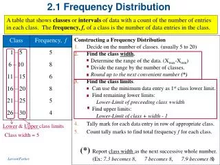
range = 73 – 50 = 23 • c.w. = 23 ÷ 6 = 3.8 → 4 • we will start the setup of the class limits with the minimum data value (50), to which we will add the class width (c.w.) • these are the lower limits (where each class begins)
Next we determine the first class’ upper limit (where it ends) by subtracting 1 from the second class’ lower limit • 54 – 1= 53 • then we add again the class width (4) to the upper class’ limits • tally
To find the class boundary we will subtract a half a unit (usually .5) from the lower class limits and add a half a unit (usually .5) to the upper class limits
We obtain the cumulative frequency by adding to the class’ frequency the frequencies of the classes above
OGIVE • Is an open line • Always rises (at least it is horizontal) • On the x-axis: class boundary • On the y-axis: cumulative frequency • Important: label the axis, name your graph