Download
1 / 23
270 likes | 459 Vues
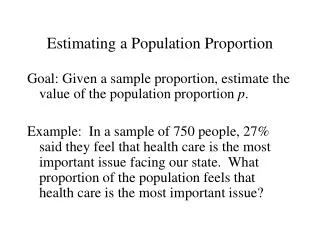
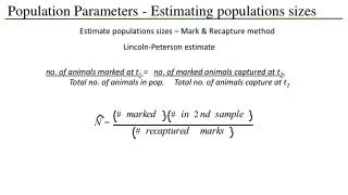
Estimating Population Parameters. Estimating Population Proportion. The sample is a simple random sample The conditions for the binomial distribution are satisfied. There are at least 5 successes and 5 failures. Requirements:.

E N D
Estimating Population Proportion • The sample is a simple random sample • The conditions for the binomial distribution are satisfied. • There are at least 5 successes and 5 failures Requirements: Fixed number of trials (n), probability of success = p, probability of failure = q, p + q = 1, trials are independent Ensures that conditions for the normal approximation of binomial distribution exist, np 5 and nq 5
Estimating Population Proportion • Let n = the size of a sample randomly chosen from a population of from which an event A will either occur or not. • Let x = the number of occurrences of event A (successes) • Let p’ = x/n the estimate of the proportion of successes in the population • Let q’ = 1- p’ proportion of failures in the sample • Ensure that x and n – x are both greater than or equal to 5 We know that a binomial distribution with np 5 and nq 5 can be approximated by a normal distribution with = np and =npq
Estimating Population Proportion From the previous result, we obtain the per-trial mean and standard deviation by dividing the mean and standard deviation of the sampling distribution by the sample size n: p = x’/n = np/n = p and p = x’ /n = (npq)/n = (pq/n)
-z/2 z/2 Estimating Population Proportion When we use a sample statistic, like p’, to estimate a population parameter, like p, we also stipulate a confidence level that expresses the probability that the population parameter lies within some interval about the estimate--the confidence interval -- to be 1 - . We usually choose to be 0.10, or 0.05, or 0.01, with the tradeoff being the higher the confidence level, 1 - , the wider the confidence interval z For the standard normal distribution, the confidence interval for a confidence level of 1- lies between the critical values, -z/2 and z/2 that are chosen such that the fraction of the area in each tail outside the critical interval is /2
Estimating Population Proportion We have previously found that the estimated per-sampleprobability of success was p’= x/n and the per-sample standard deviation was (p’q’/n) The critical value z/2 in the standard normal distribution denotes the number of standard deviations above the mean such that the fraction of the area under the curve in each tail of the curve (outside the critical interval) is /2. If we choose a confidence level of 1 - = 0.95, then 2.5% of the area lies within each tail of the curve and z/2 = 1.96 The confidence interval for for the population proportion p based upon the sample p’ is between p’ - z/2(p’q’/n) and p’ + z/2(p’q’/n) Where we take E = z/2(p’q’/n) to be the margin of errorat the 1- confidence level
Estimating Population Proportion To estimate the probability p that a given event will occur in a particular population: • Take a random sample of size n from the population and determine x, the number of occurrences of the specified event in the sample. • Let the proportion of “successes”, p’ = x/n, estimate the proportion of occurrences of the event, p, in the entire population. • Specify a confidence level, 1 - . This is the probability that the population proportion lies within a fixed interval about the measured sample proportion • From your choice of 1 - , determine z/2 the number of standard deviations from the mean such that /2 is the area in each tail outside the confidence interval. • Find the margin of error, E = z/2(p’q’/n), then state that the population proportion p lies between p’ – E and p’ + E with probability of 1 -
Estimating Population Proportion The previous analysis is valid if: • The average number of successes, x’, in a sample of size n can be approximated by a normal distribution with mean = np and standard deviation = npq
Estimating Population Proportion Example: When surveying 500 people selected at random from the general population we get 200 responses of “yes” when asked if they like broccoli. Estimate the proportion of the population that likes broccoli. p’ = x/n = 200/500 = 0.40 q’ = 1 = p’ = 0.60 np’ = 200 > 5 and nq’ = 300 > 5 normal aprox. Is OK At the 95% confidence level we have /2 = 0.025 and z/2 = 1.96 The margin for error is E = z/2(.4*.6/500) = 1.96(.022) = 0.043 P(p’- 0.043 < p < p’+ 0.043) = P(.357 < p < .443) = 0.95
Estimating Population Proportion There are two user controlled factors that determine the margin of error E = z/2(p’q’/n) (1) 1. The confidence level 1 - The smaller , the greater z/2 and the greater E 2. The sample size n The larger a value of n, the smaller E If the experimenter wants to fix the width of the confidence interval (by setting E to a pre-determined constant) and set the confidence level (by selecting a particular ), then we can use equation (1) above to determine the sample size needed to achieve this level of precision.
Estimating Population Proportion E = z/2(p’q’/n) (1) Set E and to desired values E and z/2 are constant. Solve equqtion (1) for n n =z/22(p’q’)/E2 (2) In equation (2) we have not yet taken a sample from the population, so we cannot be sure what the proportion of successes might be. The value of p’ that we use in this equation may be an estimate that we make based upon some prior knowledge, or, we may chose p’ = q’ = 0.5, which maximizes n for particular choice of and E
Estimating Population Proportion Returning to our previous example, suppose we choose = 0.05, E = 0.025, and have no prior knowledge about p’ The from equation (2) on the previous slide we obtain n =z/22(p’q’)/E2 Where z/2 =1.96 and n = (1.96)2 (0.25)/0.0252 n = 1536.4 1537
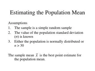
Estimating the populationmean, known • Assume: • Sample size, n > 30 • Population standard deviation is known • Then from the Central Limit Theorem, we know that the sampling distribution for samples of size n • Has mean x’ = , the mean of the original population • Has x’ = /n
Estimating the populationmean, known Let x’ be the mean of the sample of size n, then we have for a confidence interval 1 - given by P(x’ – z/2/n < < x’ + z/2/n) = 1 - Let the margin of error E =z/2/n Then with a probability of 1 - the population mean lies between x’ – E and x’ + E
x’ mean from sample of size n E E Estimating the populationmean, known If the mean were 1the probability of getting a sample x’ would be /2 1 /2 If the mean were 2the probability of getting a sample x’ would be /2 /2 2
Estimating Population mean with unknown If the population standard deviation is unknown, the sample will have to provide both an estimate on the population mean and standard deviation. Estimation of the population mean will be similar to how it was done when is known, but the sample standard deviation will be used instead. Student’s t-distribution will be used to determine the margin of error, and the confidence interval will be somewhat wider than it would be for the same sample size if were known.
Estimating Population mean with unknown Step 1. For a sample of size n, n 30, calculate the sample mean x’, and sample standard deviation s Recall: the sample variance s2 =(fixi2 – (fixi)2)/(n – 1) Step 2. Convert to a standard t-score t = (x’ - )/(s/n) Where is the (unknown) mean of both the original population and the sampling distribution Step 3. Select a confidence level 1 - , and determine t/2 Step 4. Find the margin of error E = t/2 (s/n) Then P(x’ – E x’ + E) = 1 -
Degrees of Area in One Tail freedom 0.005 0.01 0.025 0.05 ………………………………………………………. 29 2.756 2.462 2.045 1.699 Estimating Population mean with unknown Finding t/2 Choose = 0.05 , and assume n = 30 – From table A-3 Then t/2 = 2.045 for n –1 = 29 degrees of freedom
Estimating Population mean with unknown Using the TI calculator to find confidence interval for a statistic with t-distribution Let n = 106, x’ = 98.2, s = 0.62 Construct 99% Confidence Interval Step 1: Select STAT > TESTS scroll down to 8: TInterval Step 2: Select Stats if x’, n, and s are known Select Data if these values are to be calculated from a list Step 3: (Stats) Use the arrow key to move to each prompt and enter the values given above. Then Calculate <enter> Answer: TInterval (98.081, 98.319)
Estimating Population Variance Requirements: • The sample is a simple random sample • The population must have normally distributed values The sample variance has 2 distribution 2 = (n – 1) s2/2 Where n = sample size s2 = sample variance 2 = population variance (to be determined)
/2 /2 0 2 2L 2R Estimating Population Standard Deviation Confidence Interval for the Population Variance: (n-1)s2/2R < 2 < (n-1)s2/2L 2 distribution is skewed right and always positive
Area to the right of the Critical Value Degrees of Freedom 0.995 0.99 0.975 0.95 0.10 0.05 0.025 Estimating Population Standard Deviation Example: Given the following data, find the 95% confidence interval for the population standard deviation n = 41, x’ = 67200, s = 18277 P{(n-1)s2/2R < 2 < (n-1)s2/2L} = 0.95 First find 2R and 2L when each tail of the distribution contains 2.5% of the area under the curve From Table A-4 for the Chi-Square Distribution …………………………………………………………………………………………. 40 20.707 22.164 24.443 26.509 51.805 55.758 59.342
Estimating Population Standard Deviation From the previous slide we have 2R = 59.342 and 2L = 24.433 And therefore: (n-1)s2/2R = 40 (18277)2/59.342 = 2.2516 x 10⁸ and (n-1)s2/2L = 40 (18277)2/24.433 = 5.4688 x 10⁸ Thus we have: P(2.2516 x 10⁸ < 2 < 5.4688 x 10⁸) = 0.95 and for the standard deviation P(15,005 < < 23385) = 0.95